Do more parameters make a better LLM?

Parameters, context and inference effort are different dimensions. Conceptual illustration; it does not represent a particular model architecture.

Some friends were debating whether a 27B model was more intelligent than a 9B model. The intuition makes sense: with three times as many parameters, surely it must do something better. The difficulty lies in the leap from “has more” to “is better.”

Within the same family, with comparable architecture and training, the larger model usually performs better. Across families or generations, parameter count alone does not decide. That distinction gives us a useful answer: size provides a meaningful expectation when we know what we are comparing. The task and the resources we allow the model to solve it also matter.

An LLM is a large language model: a model trained to process and generate language. Let us keep those hypothetical 9B and 27B models in mind and see what changes when we open their specifications.

What does 27B parameters mean?

A parameter is a numerical value in a model that can be adjusted during training. Many are weights used in multiplications; others serve different functions. We count learned values that together represent patterns in language. Their relationship to words or facts is distributed rather than one-to-one.

Consider a small calculation: $y=w_1x_1+w_2x_2+b$. It has three adjustable parameters: two weights and a bias. The inputs change with each use; the learned values determine how they are combined. An LLM contains many operations and enormous collections of these values. This example simply helps us recognize what we are counting.

In English specifications, B means billion: one thousand million. Thus, 9B means 9 billion parameters and 27B means 27 billion. This matters when moving between languages: a billón in Spanish is a million million, or $10^{12}$. Translating 27 billion as “27 billones” multiplies the number by a thousand (Real Academia Española & ASALE, n.d. (opens in a new tab)).

More adjustable values expand representational capacity. Scaling laws describe an empirical regularity: within comparable configurations, increasing model size with sufficient data tends to reduce text prediction error. With comparable data and training recipes, that evidence favors the larger sibling in a family. This is a trend measured across models and evaluations, with diminishing returns; individual tasks still require checking the outcome (Kaplan et al., 2020 (opens in a new tab)).

The training budget—the amount of computation devoted to helping a model learn—introduces a different comparison. Chinchilla is a 70B-parameter language model introduced in a 2022 study that investigated how to divide that budget between model size and the amount of training text. It was trained on more tokens—the units into which text is divided, such as words, fragments or punctuation—than Gopher, another language model with 280B parameters. With roughly the same compute budget, Chinchilla outperformed it on many evaluations (Hoffmann et al., 2022 (opens in a new tab)). I expand on this comparison in What is an LLM, and how is it trained?, part of the AI explained series.

Across generations, the order can also reverse: a better-trained small model can outperform an older large one. Beyond more data, improvements in post-training adapt a model to tasks and instructions. One approach is distillation: training a model on examples produced by another. DeepSeek-R1 documents this procedure for transferring reasoning capabilities to smaller models (Guo et al., 2025 (opens in a new tab)). For our 9B and 27B models, comparable siblings favor the 27B version; a change in generation or recipe calls for a broader comparison.

Which models publish this information?

The models we want to compare include frontier models, those among the most capable of their time. They do not all disclose the same technical detail: their specifications may include evaluation results and usage limits without revealing internal data such as parameter counts. Before comparing figures, we need to know what information is available.

This selection includes recent models and an earlier DeepSeek release whose breakdown provides a useful example. Sources were consulted on October 4, 2026; each link leads to the developer's documentation, including model cards they publish on Hugging Face. The table separates the specifications we need to interpret.

Model and source	Declared parameters	Advertised context	Separately declared input maximum
Claude Opus 5.5 (Anthropic, n.d.-b (opens in a new tab))	Not disclosed in the consulted specification	1M tokens	—
GPT-6 Astra (OpenAI, n.d. (opens in a new tab))	Not disclosed in the consulted specification	1 050 000 tokens	922 000 tokens
Gemini 3.1 Pro Preview (Google, n.d.-a (opens in a new tab))	Not disclosed in the consulted specification	—	1 048 576 tokens
Mistral Medium 3.5 (Mistral AI, n.d. (opens in a new tab))	128B; dense architecture	256k tokens	—
Qwen3.6-35B-A3B (Qwen Team, n.d.-b (opens in a new tab))	35B total; 3B active	262 144 tokens natively	—
DeepSeek-V4-Pro, preview preceding 0813 (DeepSeek-AI, n.d.-a (opens in a new tab))	1.6T total; 49B active	1M tokens	—

A dash indicates that the consulted specification does not state that limit separately. I preserve k and M where the source abbreviates thousands or millions.

The first three rows already reveal something useful: we can compare answers, limits and costs for models whose parameter counts we do not know. Choosing a model does not require knowing its internal size. Publishing weights offers other benefits: inspecting and deploying more of the system. In either case, results establish quality. The table's limits refer to the documented versions and services; a chat application may impose different ones.

The official DeepSeek-V4-Pro-0813 release superseded this preview; note 4 explains why I retain the earlier example and how the counts differ.

How do total parameters, active parameters and layers differ?

Architecture is central to understanding a model's efficiency: it describes how its components are organized and connected, which affects the computation and memory needed to process each token. For some of the commercial models above, the public documentation offers only a partial description of that design. Dense architectures and mixtures of experts illustrate how different ways of distributing the work change the resources a network needs.

In a dense architecture, computation blocks use their weights without selecting a small group of experts for each token. In a Mixture of Experts, or MoE, certain blocks contain several alternative networks. A router calculates which ones to use for the token being processed, and their results are combined. The name might suggest a doctor, a lawyer and a programmer taking turns. These “experts” are actually subnetworks that learn different computations; their roles need not map to recognizable subjects. Mixtral’s routing analysis found no obvious assignment patterns by topic (Jiang et al., 2024, §5 (opens in a new tab)).

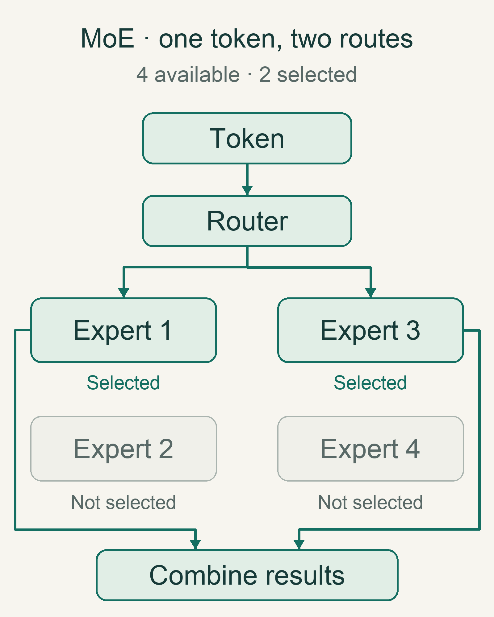
An illustrative block with four experts and two selected. It does not depict the exact architecture of any model in the table. Another token may take a different route.

Total parameters include all those weights; active parameters per token describe the portion involved in processing it, including shared components according to the model card's accounting convention. An MoE can therefore increase its total parameter count without using every expert at each step. That is its advantage. The tradeoff is keeping the weights available and managing routing and, depending on deployment, communication between devices (Jiang et al., 2024 (opens in a new tab)).

The DeepSeek-V4-Pro preview lets us follow both counts. T means trillion: its 1.6T equals 1 600B, or 1.6 billones in Spanish. This means storing the complete model requires storing its 1 600B parameters, even though 49B are active per token. Dividing 1 600 by 49 does not yield a reliable speed multiplier relative to a 1 600B dense model: attention, memory, communication and hardware also matter. Its model card specifies FP4 for experts and FP8 for most other parameters. Storage depends both on how many values we retain and on their representation.

Layers count successive processing stages. An MoE block can sit inside a layer. Qwen3.6-35B-A3B, for example, declares 40 layers and, within its MoE blocks, 8 active routed experts plus one shared expert. That means 9 experts per MoE block for each token, not 9 active layers or 3 billion layers (Qwen Team, n.d.-b (opens in a new tab)). When “effective layers” appears, we need to know the definition being used.

Qwen also lets us compare models from the same generation. Its Qwen3.6-27B card reports 59.3 for that dense model versus 51.5 for Qwen3.6-35B-A3B on Terminal-Bench 2.0, a test of terminal work; on SWE-bench Verified, a test of software issue resolution, the scores are 77.2 versus 73.4. The dense model leads in both. These are developer-reported results under its evaluation conditions. We have held generation constant, while architecture and size still differ: 27B dense parameters versus 35B total and 3B active in the MoE. The comparison illustrates why total parameters alone cannot rank quality: the MoE contains more yet trails in both tests (Qwen Team, n.d.-a (opens in a new tab)).

We now have two separate questions: how much the model contains and how much it uses per token. To know whether it fits on our computer, we need a third: how those numbers are stored.

Do more parameters require more memory?

With the same numerical representation, storing more parameters requires more space. But different versions do not necessarily store each weight with the same number of bits. Quantization reduces the precision used to represent certain values to save memory; it can affect quality, with consequences that depend on the method and task. A quantized model can retain the same parameter count. OPTQ, which first circulated as GPTQ, is one method for quantizing already-trained weights (Frantar et al., 2023 (opens in a new tab)).

Returning to 9B and 27B, we can calculate idealized weight storage using decimal GB:

Hypothetical case	Calculation	Weights only
9B at 16 bits	$9\times10^9\times16/8$ bytes	18 GB
27B at 16 bits	$27\times10^9\times16/8$ bytes	54 GB
27B at 4 bits	$27\times10^9\times4/8$ bytes	13.5 GB

The larger model can use less space for weights if we represent them with fewer bits. Complete RAM or VRAM requirements also include quantization metadata, temporary memory and the state needed to process the context. Note 1 explains those components and the difference between GB and GiB.

For otherwise comparable dense models, more parameters usually require more computation per token. Actual runtime also depends on architecture and implementation. Quantization can enable a run that previously did not fit in memory; its usefulness depends on the resulting quality and hardware support. When we use an API, some of this engineering sits with the service, and we assess it through its limits, response times and costs.

Does a larger context window help a model use documents better?

Parameters belong to the learned model. Context is the information available during a run: instructions, conversation, documents and tool results, along with the space generation requires under the service's rules. A document supplied with a request enters that context; retaining it for other conversations requires an additional product mechanism. During execution, a larger context usually takes more memory for the attention cache, connecting it to the RAM or VRAM discussed above (Anthropic, n.d.-a (opens in a new tab)).

That space is measured in tokens, the text processing units we encountered when discussing training. Their equivalent in words or pages depends on the tokenizer. Images and other media have their own accounting rules. For a real workload, the model's token counter provides the relevant measure (Google, n.d.-b (opens in a new tab)).

A wide window allows more material to be supplied at once. The output limit tells us how much the model can generate. GPT-6 Astra declares all three limits: 1 050 000 tokens of context, 922 000 of input and 128 000 of output. Its input limit equals context minus maximum output. For output, Claude Opus 5.5 declares 128K for standard requests or 300K through the Batch API in beta; Gemini 3.1 Pro Preview, 65 536. These limits differ from context or input limits. Note 2 shows how to budget input and generation, including reasoning that uses the same space.

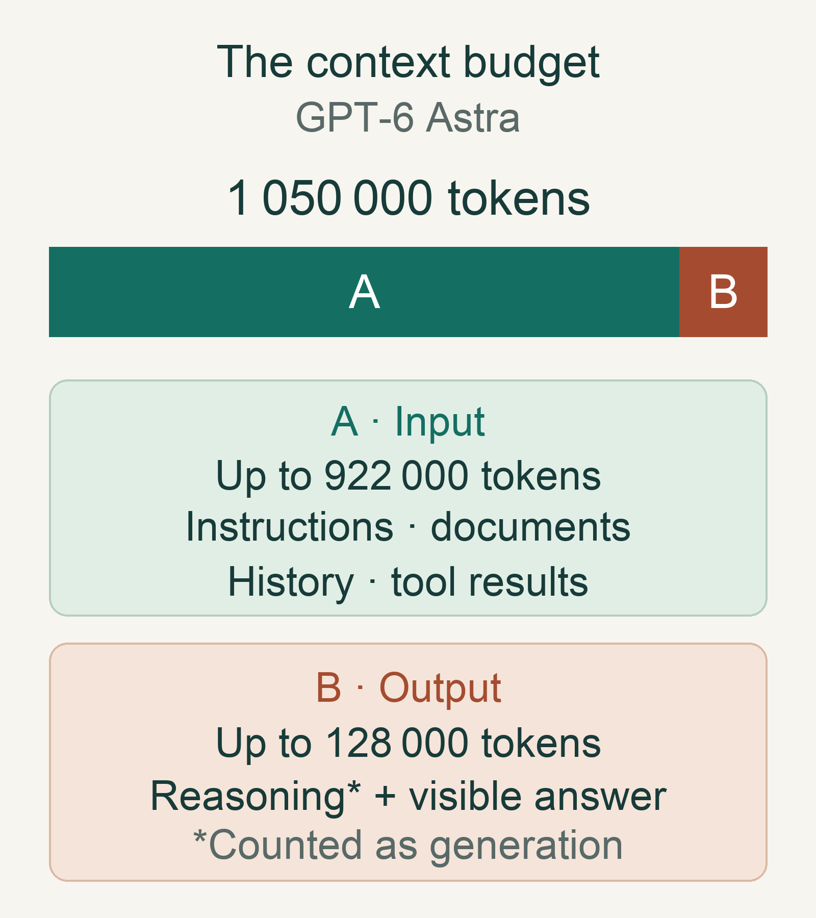
GPT-6 Astra's declared maxima, drawn to scale (OpenAI, n.d. (opens in a new tab)). With 900 000 input tokens, 150 000 remain in the context, but the output cap stays at 128 000. The diagram shows capacity; how effectively the content is used requires separate evaluation.

Suppose we need to find contradictions across several reports. A larger window lets us include more documents; using them requires connecting their passages. Lost in the Middle, published in 2024 with evaluations of 2023 models, showed that information position affected performance (Liu et al., 2024 (opens in a new tab)). NoLiMa, published at ICML 2025, added a test with little shared wording between a question and the relevant passage. At 32K tokens, 11 of the 13 evaluated models fell below half their short-context performance. Finding associations became harder as the material grew, even when the supported context was much larger (Modarressi et al., 2025 (opens in a new tab)).

For our reports, we would vary position, length and vocabulary overlap: questions with evidence at the beginning, middle and end; short and long versions of the documents; questions describing an idea in different words from the passage. We would also include contradictions requiring several fragments to be combined. This measures whether the model uses the available space effectively for the work we need.

Why can the same model answer better if it takes longer?

Training determines the weights. At response time, during inference, we can also allocate more computation. Mistral Medium 3.5 allows reasoning effort to be configured per request with the same weights (Mistral AI, n.d. (opens in a new tab)).

In a model that reasons through intermediate text, generation continues before the final answer: it proposes steps, calculates and may revise an attempt. In ordinary autoregressive decoding, each new token requires another pass through the model, reusing the attention cache; the preceding sequence becomes input to the next step. More steps provide more sequential computation with the same parameters. Qwen's model card shows this separation between reasoning content and the answer (Qwen Team, n.d.-b (opens in a new tab)).

The DeepSeek-V4-Pro preview lets us observe the effect within one model. On GPQA Diamond, its developer reports 72.9 in Non-Think mode, 89.1 in High and 90.1 in Max. The gains shrink from 16.2 to 1.0 percentage points, recalling the diminishing improvements discussed under scaling. We also need to consider the ceiling effect: around 90 out of 100, less room remains for improvement. The outcome depends on the test; effort labels are system-specific controls, so these steps need not represent equal increments of computation (DeepSeek-AI, n.d.-a (opens in a new tab)).

We can return to our 9B and 27B models. On a multi-step problem, allowing the 9B model to develop and revise a solution could change the outcome against the 27B model giving a direct answer. This is a hypothesis we would test with those models, not a measurement made here. A useful comparison records accuracy, waiting time and consumption: extra effort is worth the improvement it brings to our task.

When discussing speed, we need to distinguish time until a useful answer begins, generation speed and time until completion. A service may generate many tokens per second after a long wait. Artificial Analysis even distinguishes the first reasoning token from the first token of the final answer (Artificial Analysis, n.d.-b (opens in a new tab)).

Cost per task combines how much we send, how much the model generates, which reasoning is billed and how many attempts or tools we need. Note 3 works through hypothetical rates. With those components, we can compare cost per correct answer alongside prices per million tokens.

So how do I choose an LLM?

Once we understand the numbers, we need to give them a concrete job. To compare reports in Spanish, I would start with a small set of documents and questions whose answers I can check. I would include contradictions, information spread across documents and questions the documents cannot answer. That lets us observe both correct results and invented answers.

Specifications help eliminate incompatibilities: insufficient context, output that is too short or a modality that cannot accept our files. Gemini 3.1 Pro Preview, for example, documents text, image, audio, video and PDF input, with text output. Both directions deserve checking when a specification says “multimodal.” After that filter, I would compare:

• Task quality: correct answers, evidence that actually supports them and instruction following. Executable tests for code; verifiable passages for documents.
• Execution conditions: exact version, reasoning effort, tools and quantization where applicable. A result describes the conditions under which it was obtained.
• Required resources: time to the complete answer, cost per resolved case and, for local execution, memory and hardware.
• Terms of use: data handling, deployment options and the applicable license. Access to weights does not imply an absence of restrictions.

A benchmark, or set of evaluation tests, can inform the initial selection. Its score summarizes specific tests and conditions. The Artificial Analysis Intelligence Index evaluates text in English; the organization separately publishes a Multilingual Index based on Global-MMLU-Lite that includes Spanish. The latter is closer to our working language, although our reports and prepared questions remain the decisive test (Artificial Analysis, n.d.-a (opens in a new tab)).

We can now return to the conversation between friends with a more precise answer. If 9B and 27B are siblings with comparable architecture, data and training, the larger model starts with a favorable expectation of quality, at a greater resource cost. If generation, architecture or reasoning effort differs, we need to examine those differences: a smaller model may be better for the task. Specifications help us frame a fair comparison; our tests turn that expectation into a decision.

Notes

1. Weight storage and runtime memory. The approximation is $M=P\times b/8$ bytes, where $P$ is the parameter count and $b$ the bits per parameter. It assumes uniform precision and excludes scales or other metadata. Here, 1 GB equals $10^9$ bytes; 1 GiB equals $2^{30}$ bytes. Generation commonly maintains a key–value (KV) cache to reuse attention computations. Its size depends on context, architecture, precision and concurrent requests. Caches can be compressed or moved between devices, with consequences for memory and speed (Hugging Face, n.d.-a (opens in a new tab)). On a GPU with 16 GiB, about 17.2 decimal GB, 13.5 GB of weights would leave about 3.7 GB for the other components. Whether that is enough depends on the run. Return to the calculation.
2. Budgeting input and output with a real specification. GPT-6 Astra publishes 1 050 000 context tokens, a maximum input of 922 000 and a maximum output of 128 000. The sum $922\,000+128\,000=1\,050\,000$ joins the three declared limits: the input maximum equals the space left when reserving maximum output. With 900 000 input tokens, 150 000 would remain in the context, while the output cap would still be 128 000. Reasoning counted as generation shares that output budget with the visible answer. The Markdown version of the model page lists the three figures explicitly (OpenAI, n.d. (opens in a new tab)). Return to context.
3. Rates and total cost. At hypothetical prices of USD 2 per million input tokens and USD 10 per million output tokens, a request with 10 000 input tokens and 1 000 billed output tokens would cost $0.01\times2+0.001\times10=0.03$ USD. That is three cents under those conditions. The calculation excludes tools, discounts, caching and any other fees; if reasoning is billed as output, its tokens must be included. The rates serve only this example. Return to costs.
4. Which DeepSeek package are we counting? The official DeepSeek-V4-Pro-0813 release supersedes the preview and adds the DSpark speculative decoding module (DeepSeek-AI, n.d.-b (opens in a new tab)). On the consultation date, the Hugging Face API’s safetensors.total field returned 1 650 497 936 906 for 0813, approximately 1.65T, versus 1 598 839 674 782 for the preview, approximately 1.60T (Hugging Face, n.d.-b (opens in a new tab); Hugging Face, n.d.-c (opens in a new tab)). The interface rounds the former to 1.7T. These are repository tensor counts obtained by the same method; attributing the entire difference to a particular module would require a component breakdown. I retain the identified preview because its card documents both total and active parameters and the three reasoning modes compared here. Return to the table.

References

Anthropic. (n.d.-a). Context windows. Claude API Docs. Retrieved October 4, 2026, from Original source (opens in a new tab)

Anthropic. (n.d.-b). Opus 5.5. Claude API Docs. Retrieved October 4, 2026, from Original source (opens in a new tab)

Artificial Analysis. (n.d.-a). Artificial Analysis Intelligence Index. Retrieved October 4, 2026, from Original source (opens in a new tab)

Artificial Analysis. (n.d.-b). Language model API performance benchmarking. Retrieved October 4, 2026, from Original source (opens in a new tab)

DeepSeek-AI. (n.d.-a). DeepSeek-V4-Pro [Model card]. Hugging Face. Retrieved October 4, 2026, from Model card (opens in a new tab)

DeepSeek-AI. (n.d.-b). DeepSeek-V4-Pro-0813 [Model card]. Hugging Face. Retrieved October 4, 2026, from Model card (opens in a new tab)

Frantar, E., Ashkboos, S., Hoefler, T., & Alistarh, D. (2023). OPTQ: Accurate post-training quantization for generative pre-trained transformers. In The Eleventh International Conference on Learning Representations. Published version, institutional repository (opens in a new tab)

Google. (n.d.-a). Gemini 3.1 Pro Preview. Google AI for Developers. Retrieved October 4, 2026, from Original source (opens in a new tab)

Google. (n.d.-b). Understand and count tokens. Google AI for Developers. Retrieved October 4, 2026, from Original source (opens in a new tab)

Guo, D., Yang, D., Zhang, H., Song, J., Wang, P., Zhu, Q., Xu, R., Zhang, R., Ma, S., Bi, X., Zhang, X., Yu, X., Wu, Y., Wu, Z. F., Gou, Z., Shao, Z., Li, Z., Gao, Z., Liu, A., . . . Zhang, Z. (2025). DeepSeek-R1 incentivizes reasoning in LLMs through reinforcement learning. Nature, 645, 633–638. DOI (opens in a new tab)

Hoffmann, J., Borgeaud, S., Mensch, A., Buchatskaya, E., Cai, T., Rutherford, E., de Las Casas, D., Hendricks, L. A., Welbl, J., Clark, A., Hennigan, T., Noland, E., Millican, K., van den Driessche, G., Damoc, B., Guy, A., Osindero, S., Simonyan, K., Elsen, E., . . . Sifre, L. (2022). An empirical analysis of compute-optimal large language model training. In S. Koyejo, S. Mohamed, A. Agarwal, D. Belgrave, K. Cho, & A. Oh (Eds.), Advances in Neural Information Processing Systems (Vol. 35, pp. 30016–30030). Curran Associates. DOI (opens in a new tab)

Hugging Face. (n.d.-a). Cache strategies. Transformers. Retrieved October 4, 2026, from Original source (opens in a new tab)

Hugging Face. (n.d.-b). DeepSeek-V4-Pro [Safetensors metadata]. Retrieved October 4, 2026, from API record (opens in a new tab)

Hugging Face. (n.d.-c). DeepSeek-V4-Pro-0813 [Safetensors metadata]. Retrieved October 4, 2026, from API record (opens in a new tab)

Jiang, A. Q., Sablayrolles, A., Roux, A., Mensch, A., Savary, B., Bamford, C., Chaplot, D. S., de las Casas, D., Hanna, E. B., Bressand, F., Lengyel, G., Bour, G., Lample, G., Lavaud, L. R., Saulnier, L., Lachaux, M.-A., Stock, P., Subramanian, S., Yang, S., . . . El Sayed, W. (2024). Mixtral of experts [Preprint]. arXiv. arXiv (opens in a new tab)

Kaplan, J., McCandlish, S., Henighan, T., Brown, T. B., Chess, B., Child, R., Gray, S., Radford, A., Wu, J., & Amodei, D. (2020). Scaling laws for neural language models [Preprint]. arXiv. arXiv (opens in a new tab)

Liu, N. F., Lin, K., Hewitt, J., Paranjape, A., Bevilacqua, M., Petroni, F., & Liang, P. (2024). Lost in the middle: How language models use long contexts. Transactions of the Association for Computational Linguistics, 12, 157–173. DOI (opens in a new tab)

Mistral AI. (n.d.). Mistral Medium 3.5 128B [Model card]. Hugging Face. Retrieved October 4, 2026, from Model card (opens in a new tab)

Modarressi, A., Deilamsalehy, H., Dernoncourt, F., Bui, T., Rossi, R. A., Yoon, S., & Schuetze, H. (2025). NoLiMa: Long-context evaluation beyond literal matching. In A. Singh, M. Fazel, D. Hsu, S. Lacoste-Julien, F. Berkenkamp, T. Maharaj, K. Wagstaff, & J. Zhu (Eds.), Proceedings of the 42nd International Conference on Machine Learning (Vol. 267, pp. 44554–44570). PMLR. Proceedings (opens in a new tab)

OpenAI. (n.d.). GPT-6 Astra. OpenAI API. Retrieved October 4, 2026, from Original source (opens in a new tab) · Markdown version (opens in a new tab)

Qwen Team. (n.d.-a). Qwen3.6-27B [Model card]. Hugging Face. Retrieved October 4, 2026, from Model card (opens in a new tab)

Qwen Team. (n.d.-b). Qwen3.6-35B-A3B [Model card]. Hugging Face. Retrieved October 4, 2026, from Model card (opens in a new tab)

Real Academia Española & Asociación de Academias de la Lengua Española. (n.d.). Billón. In Diccionario panhispánico de dudas (2nd ed.). Retrieved October 4, 2026, from Dictionary entry (opens in a new tab)