What is an LLM, and how is it trained?

Let’s write “The fisherman repaired his net.” Cover the last word and leave “The fisherman repaired his…” visible. You might have thought of “net,” although “boat” could work too. We can picture the fisherman beside the water. To train a language model, that scene becomes something a computer can calculate: distribute probabilities among possible continuations and compare them with what the text actually said.

A sentence, a continuation to anticipate and several attempts at adjustment. A conceptual watercolor; the cards and corrections represent the exercise, not a model’s internal calculations.

In the Transformer article, we followed this fisherman while his sentence was translated. We have also seen how the training material is prepared. Now we will see how a model learns to anticipate a continuation. Having an architecture and a collection of texts still leaves a task to solve: finding the numerical values with which that architecture will make useful predictions.

By the end, you will be able to distinguish the data, objective, architecture and trained model, and follow a pretraining cycle: what goes in, what is predicted, how the difference is measured and what changes afterward. We will keep the fisherman with us along the way. You do not need to have read the whole series; we will bring each idea back when we need it.

A model of possible continuations

A language model assigns probabilities to sequences of tokens, the units into which text is divided for processing. In the kind we will follow here, it calculates the distribution of the next token given the preceding ones. That makes it possible to score a continuation and, later, produce text.

Language modeling already had a history before the networks we are following here. N-gram models estimated continuations from short word sequences observed in texts, combining contexts of different lengths to handle new cases (Bengio et al., 2003, section 1 (opens in a new tab)). Against that background, Yoshua Bengio and his coauthors presented a model at NIPS 2000 that jointly learned word representations and sequence probabilities; an expanded version appeared in JMLR in 2003 (Bengio et al., 2000 (opens in a new tab); 2003 (opens in a new tab)). Sharing representations allowed one sentence to inform predictions for others containing words with nearby representations, even when the complete sequence was new.

LLM stands for large language model. The term usually refers to networks with many parameters, trained on large amounts of text. “Large” describes a scale; there is no single number marking a universal boundary. Parameters are the network’s adjustable numbers. Their count, the tokens used for training and the computation expended describe different aspects of that scale.

To make the journey concrete, we will choose a decoder-only Transformer: the variant we met when moving from translation to models that continue text. Here, the same sequence supplies the context for predicting the next token, without a separate encoder to consult. This is an autoregressive model. GPT-2 is a documented example of this choice (Radford et al., 2019, section 2 (opens in a new tab)). Other designs and training objectives exist; this will be our route through the mechanism.

The sentence carries its own reference

Let’s return to “The fisherman repaired his net.” To see how examples are prepared, imagine a teaching tokenizer that keeps each word as one token and separates the final period. We will leave spaces out of the diagram. A real tokenizer may split words differently; what matters here is the relationship between the input and what should follow.

Text available for prediction	Next token in the document
The	fisherman
The fisherman	repaired
The fisherman repaired	his
The fisherman repaired his	net
The fisherman repaired his net	.

One sentence supplies several positions at which to compare a prediction with a reference. The target token is the one that actually comes next in the document. When preparing training, the program already knows it: it comes from shifting the same token sequence by one position.

This is why we call it self-supervised learning. We do not need someone to write a separate answer for each prefix; we can obtain it from the material. Work such as the GPT-2 report described this as unsupervised learning, as its title reflects; “self-supervised” emphasizes where the targets come from. The human decisions about which texts to include are still there, as we saw in the previous article.

Nor does the reference declare “net” the only reasonable continuation. In another sentence the fisherman might repair his boat. This example supplies one observation; others supply different ones, and their frequencies and contexts will also influence learning. The procedure seeks to fit a distribution, rather than write a rule requiring the same final word every time.

Seeing the sentence without reading ahead

Before learning, we need to get the network running. In training from scratch, many weight matrices start with random values chosen according to an initialization rule; other parameters may start at fixed values. A structure capable of computation already exists, but its predictions do not yet reflect what we want it to learn from the corpus.

The forward pass begins with token identifiers selecting rows from an embedding table, their numerical representations. Positional information and the Transformer blocks transform those representations. For the prefix “The fisherman repaired his,” the output at the last position brings together information the network will use to score possible continuations.

An output projection produces a score, or logit, for each token in the vocabulary. Softmax converts those scores into positive probabilities that sum to one.

For a baseline, take a hypothetical vocabulary with 50 257 entries, the size documented for GPT-2 (Radford et al., 2019, section 2.3 (opens in a new tab)). With equal logits, softmax distributes probability uniformly: each token receives $1/50\,257\approx0.00002$. With logits very close to one another, the distribution would be nearly uniform. This mathematical reference gives us a scale; a newly initialized network’s logits depend on its design and initialization.

Now let’s construct a more concentrated hypothetical distribution so we can follow the calculations. We will assign 0.10 to “net” for convenience, without attributing these numbers to a particular training stage:

Continuation	Probability
net	0.10
boat	0.45
basket	0.25
All other tokens combined	0.20

The last row groups many alternatives; the model scores every token separately.

There seems to be a loophole: if the program has the complete sentence, how do we prevent the network from looking at “net” before predicting it? The causal mask we used in the Transformer walkthrough returns here: it prevents each position from attending to later positions. The output at “his” can use “The fisherman repaired his,” but not the “net” or period that follow. The original Transformer describes this restriction together with shifting the outputs during training (Vaswani et al., 2017, section 3.1 (opens in a new tab); manuscript detail (opens in a new tab)).

Because the reference prefixes are already available, a causal Transformer can compute predictions for many positions in parallel, respecting the mask in each layer. To calculate the prediction after “net,” it uses the document’s “net,” even if its previous prediction favored “boat.” Using the reference tokens as context during training is known as teacher forcing (Goodfellow et al., 2016, section 10.2.1 (opens in a new tab)). Each comparison therefore starts from the prefix supplied by the document.

Putting a number on the difference

Our distribution gives “net” a probability of only 0.10. We now need a measure that distinguishes it from one assigning 0.60. Reporting only “right” or “wrong” would lose information about how much support the reference receives.

The loss function turns that comparison into a number. We will use cross-entropy with a single target token: it takes the probability assigned to that token and transforms it so that a low probability produces a high loss. The PyTorch documentation presents the operation starting from logits (PyTorch contributors, n.d. (opens in a new tab)).

In the uniform baseline, the loss for any target token would be $-\ln(1/50\,257)$, or $\ln(50\,257)\approx10.825$. That is our numerical point of comparison.

Using natural logarithms, assigning 0.10 to “net” gives a loss of approximately 2.303; assigning 0.60 gives approximately 0.511. These are two hypothetical distributions we are comparing, not a guaranteed improvement after one update. Note 1 develops the formula and the average for a sequence.

That loss measures something quite specific: how much support the observed token received. If the document contained a false statement, the calculation would still have a reference. In our example we know what the person wrote; establishing whether a fisherman actually repaired a net would be another task. This distinction sets a concrete limit on what we can conclude when loss falls.

The error reaches the numbers that can change

So far, the network has made a prediction and received a measure of its disagreement with the text. Now we return to the loss, gradient and update cycle from the neural-network article: there, we changed weights that helped recognize a 3; here, we will adjust those involved in anticipating the fisherman’s next word.

Backpropagation calculates how the loss would respond to small changes in the parameters involved in the computation. Those derivatives form the gradient. We can read them as local indications: increasing one number would tend to raise the loss; increasing another would tend to lower it. The optimizer uses those indications to decide the update.

With gradient descent, we take a step in the direction that reduces loss according to that local estimate. The learning rate controls its size. Too large a step can undo the improvement we expected; too small a step can make progress slow. A general explanation of this cycle is developed in Goodfellow et al. (2016, chapter 8) (opens in a new tab).

We can isolate one weight in the output projection to observe it. In the numerical example in note 2, that weight goes from 0.400 to 0.418. If we hold everything else fixed, the probability of “net” rises from 0.10 to approximately 0.1033. The adjustment is small, but we can already point to what changed and recalculate its effect.

In full training, gradients can also reach the embeddings and the transformations in attention and the other layers. Learning can change both the representations and the way they are combined. Weights are shared across many contexts: an update prompted by the fisherman may affect other sentences. In general, there is no isolated parameter we can interpret as “knowing how to repair nets.”

The gradient descent step we just used is one simple option. Adam, for instance, maintains estimates of gradients and their squares to adapt updates (Kingma & Ba, 2015 (opens in a new tab)). Those estimates change the step sizes applied to different parameters; we still use gradients of the same loss function.

One sentence shares its update with many others

If we only repeated our sentence, we could improve that prediction without building a model useful for much else. Now place beside it “The fisherwoman put away her net,” “The mechanic repaired his engine” and “The girl repaired her kite.” These are invented examples, but they reveal the difficulty: some contexts share an activity, others a person or an object, and the continuations change.

Different sentences can contribute to updates of the same parameters. A conceptual watercolor of our text examples.

In practice, sequences are assembled into a batch. Losses from their valid positions are combined, and gradients are calculated for that joint objective. Instead of correcting each sentence separately, the update combines their contributions. Positions added solely as padding can be excluded from the loss.

Our cycle is now: prepare a batch, calculate its distributions, compare them with the reference tokens, obtain gradients and update the parameters. Then another batch arrives and the cycle repeats. A training step usually refers to one optimizer update; it may bring together several small batches through gradient accumulation. An epoch is one pass through the training set, although with very large collections progress is also described by counting the tokens processed.

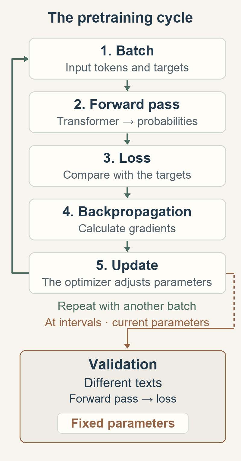
The training loop changes parameters. At intervals, a separate validation pass measures loss on other texts with those parameters held fixed.

We call this general learning stage pretraining because it can provide a basis for later uses and adjustments. The task of anticipating tokens repeats across varied texts; to reduce its loss, the network can learn regularities useful in many contexts. Whether a regularity emerges, is memorized or is applied successfully to a new case is something we need to check.

Checkpoints are saved at intervals. To run the model, we need its configuration and learned parameters, together with the matching tokenizer. Faithfully resuming training requires preserving more state, including the optimizer’s. The architecture describes the operations; the saved parameters reflect the training already carried out.

What grows when an LLM grows

Now imagine expanding that work. We can increase the parameter count, present more tokens or spend more computation. The three decisions are connected: a larger network costs more per step, and processing more text requires more operations. Adding parameters also leaves more values to fit using the available examples.

The study known as Chinchilla examined how to divide a compute budget between model size and amount of training. Its 70-billion-parameter model processed 1.4 trillion tokens; Gopher, with 280 billion parameters, had processed 300 billion. The compute budget was approximately the same (Hoffmann et al., 2022, table 1 (opens in a new tab)).

Take one concrete comparison: on MMLU, a collection of questions across 57 academic subjects, the 5-shot evaluation—with five examples in the context—gave an average accuracy of 67.6% for Chinchilla versus 60.0% for Gopher, a difference of 7.6 percentage points. Chinchilla improved on 51 tasks, tied on two and performed worse on four (Hoffmann et al., 2022, section 4.2 (opens in a new tab); supplementary tables A8–A9 (opens in a new tab)). The comparison showed that Gopher was undertrained for its compute budget: a smaller model trained on more tokens made better use of roughly the same computation.

That balance changes when we also count the cost of using the model. The analysis by Sardana et al. (2024) (opens in a new tab) shows that, with enough inference demand, training a smaller model for longer can be worthwhile: the extra training work is offset when serving requests. The authors point to the 15 trillion tokens used for Llama 3 as an example of training far beyond the training-only Chinchilla criterion. The economic objective now includes later use.

Also, counting processed tokens does not tell us how many were distinct: making ten passes over the same material adds work without adding ten new collections. The repetitions and source mixtures we considered when preparing data matter again here.

In our case, increasing the count by copying the fisherman’s sentence would be easy. The harder, more interesting work would be gathering other uses of language that let us test which relationships the model manages to learn.

Improvement has to leave the practice notebook

We can watch loss fall on the training batches. But we want to know what happens with texts we did not use to adjust the weights. That is why we also calculate loss on validation material, running the model without updating its parameters from those examples.

The practice notebook and the reserved texts serve different purposes. Validation measures loss while parameters stay fixed. A conceptual watercolor.

Suppose it improves greatly at completing “The fisherman repaired his net” but barely improves on new sentences. That would give us reason to investigate overfitting: adaptation to the particularities of training that does not extend as we hoped. We would also need to check whether validation represents a different distribution. Distinguishing those causes requires examining the texts and evaluation conditions alongside the curves.

Language modeling also uses perplexity, a transformation of average loss. With the same tokenizer, texts and procedure, lower perplexity indicates that the model assigned higher probability to the observed continuations. Note 3 explains the relationship. The measure is not a percentage of correct answers, nor does it establish that the model is a good assistant.

Let’s return to a concrete decision. If we want to use it to answer questions about fishing, completing sentences from a manual well provides evidence about a limited capability. We will also need questions and criteria for checking whether the answers are correct and useful. The training objective tells us what was optimized; evaluating the intended use tells us how far that learning reached.

When we really remove the word

At the end of pretraining we have a base model with adjusted parameters. We can write “The fisherman repaired his” again and calculate a distribution using those values. This time there is no reference token waiting for us to measure the loss: we want a continuation.

In this ordinary inference, parameters remain fixed. We choose a token through a selection rule, append it to the input and calculate the next distribution. That is the difference from teacher forcing: after the initial text, the context incorporates the continuations we have just generated. The available text changes, and so do the internal representations, even without a weight update. Training modified the mechanism; now we are using it.

There is still distance between continuing text and responding well to a request. The InstructGPT study, for instance, examined later adjustments using human demonstrations and preferences to guide that behavior (Ouyang et al., 2022 (opens in a new tab)). That will be another question in this series. First, we will follow how a distribution becomes a response, token by token.

The opening sentence still fits on a single line. Now we can recognize what happened around it: the text supplied the references, the architecture calculated predictions, the objective measured a difference and the optimizer adjusted parameters. The LLM we have followed is, in the end, a decoder-only Transformer whose parameters result from repeating that cycle over many texts. It uses those parameters to calculate probabilities for continuing a sequence. When “net” appears on the screen, we will see a word; behind its probability will be a history of examples and small changes that we now know how to begin reconstructing.

Notes

1. From probability to loss. For a target token $y$, with probability $p_\theta(y\mid x)$ given prefix $x$, we use $\ell=-\ln p_\theta(y\mid x)$. The symbol $\theta$ collects the parameters. Thus, $-\ln(0.10)\approx2.303$ and $-\ln(0.60)\approx0.511$. For a sequence $x_1,\ldots,x_T$ with $T\ge2$, if we score from the second token onward and give each position equal weight:

   $$L(\theta)=-\frac{1}{T-1}\sum_{t=2}^{T}\ln p_\theta(x_t\mid x_1,\ldots,x_{t-1})$$

   The denominator counts the positions evaluated. With a start token, we could score the first one too. For a batch, the average must respect valid positions and the chosen weights. In this case without label smoothing, minimizing cross-entropy is equivalent to maximizing the log-likelihood of the observed continuations (Goodfellow et al., 2016, section 6.2.1.1 (opens in a new tab); PyTorch contributors, n.d. (opens in a new tab)). Return to the comparison.

2. A weight we can actually follow. We isolate a weight $w$ connecting a fixed activation $h=2$ to the logit for “net”: $z_{\mathrm{net}}=wh+c$, where $c$ collects the remaining contributions, which we will hold fixed. We take $w=0.400$ and choose those contributions and the other logits so that the initial probability is $p_{\mathrm{net}}=0.10$. For softmax and the loss targeting “net,” $\partial\ell/\partial z_{\mathrm{net}}=p_{\mathrm{net}}-1=-0.90$. By the chain rule:

   $$\frac{\partial\ell}{\partial w}=(0.10-1)\cdot2=-1.8$$

   With learning rate $\eta=0.01$, one gradient descent step gives:

   $$\begin{aligned} w'&=w-\eta\frac{\partial\ell}{\partial w}\\ &=0.400-0.01(-1.8)\\ &=0.418 \end{aligned}$$

   The logit increases by $(0.418-0.400)\cdot2=0.036$. Holding the other logits and all activations fixed, the new probability is:

   $$\begin{aligned} p'_{\mathrm{net}}&=\frac{0.10e^{0.036}}{0.90+0.10e^{0.036}}\\ &\approx0.1033 \end{aligned}$$

   This is a teaching calculation with a single free weight, no regularization and no additional shared parameters. A real update combines gradients from many positions and can change many probabilities at once; it does not guarantee improvement on every example. The softmax gradient corresponds, with the opposite sign when maximizing log-likelihood, to the calculation in Bengio et al. (2003, pp. 1145–1146) (opens in a new tab). Return to the update.

3. What perplexity expresses. If $L$ is average loss per token calculated with natural logarithms, perplexity is $\mathrm{PPL}=e^L$. For example, $L=\ln 4$ corresponds to a perplexity of 4. It equals the inverse geometric mean of the probabilities assigned to observed tokens; it does not mean there were exactly four candidates at every position. Bengio et al. (2003, p. 1141) (opens in a new tab) describe this measure for reporting their language-modeling results. Changing the tokenizer changes the unit being averaged; the GPT-2 report discusses this comparison difficulty (Radford et al., 2019, section 3.1 (opens in a new tab)). Return to validation.

References

Bengio, Y., Ducharme, R., & Vincent, P. (2000). A neural probabilistic language model. In T. K. Leen, T. G. Dietterich, & V. Tresp (Eds.), Advances in Neural Information Processing Systems (Vol. 13, pp. 932–938). MIT Press. Conference proceedings (opens in a new tab)

Bengio, Y., Ducharme, R., Vincent, P., & Jauvin, C. (2003). A neural probabilistic language model. Journal of Machine Learning Research, 3, 1137–1155. Original paper (opens in a new tab)

Goodfellow, I., Bengio, Y., & Courville, A. (2016). Deep learning. MIT Press. Complete book (opens in a new tab)

Hoffmann, J., Borgeaud, S., Mensch, A., Buchatskaya, E., Cai, T., Rutherford, E., de Las Casas, D., Hendricks, L. A., Welbl, J., Clark, A., Hennigan, T., Noland, E., Millican, K., van den Driessche, G., Damoc, B., Guy, A., Osindero, S., Simonyan, K., Elsen, E., . . . Sifre, L. (2022). An empirical analysis of compute-optimal large language model training. In S. Koyejo, S. Mohamed, A. Agarwal, D. Belgrave, K. Cho, & A. Oh (Eds.), Advances in Neural Information Processing Systems (Vol. 35, pp. 30016–30030). Curran Associates. Conference proceedings (opens in a new tab) DOI (opens in a new tab)

Kingma, D. P., & Ba, J. (2015). Adam: A method for stochastic optimization [Paper presentation]. 3rd International Conference on Learning Representations, San Diego, CA, United States. Author manuscript (opens in a new tab)

Ouyang, L., Wu, J., Jiang, X., Almeida, D., Wainwright, C. L., Mishkin, P., Zhang, C., Agarwal, S., Slama, K., Ray, A., Schulman, J., Hilton, J., Kelton, F., Miller, L., Simens, M., Askell, A., Welinder, P., Christiano, P. F., Leike, J., & Lowe, R. (2022). Training language models to follow instructions with human feedback. In S. Koyejo, S. Mohamed, A. Agarwal, D. Belgrave, K. Cho, & A. Oh (Eds.), Advances in Neural Information Processing Systems (Vol. 35, pp. 27730–27744). Curran Associates. Conference proceedings (opens in a new tab) DOI (opens in a new tab)

PyTorch contributors. (n.d.). CrossEntropyLoss. PyTorch 2.9 documentation. Retrieved October 4, 2026, from the project documentation (opens in a new tab).

Radford, A., Wu, J., Child, R., Luan, D., Amodei, D., & Sutskever, I. (2019). Language models are unsupervised multitask learners [Technical report]. OpenAI. Original report (opens in a new tab)

Sardana, N., Portes, J., Doubov, S., & Frankle, J. (2024). Beyond Chinchilla-optimal: Accounting for inference in language model scaling laws. In R. Salakhutdinov, Z. Kolter, K. Heller, A. Weller, N. Oliver, J. Scarlett, & F. Berkenkamp (Eds.), Proceedings of the 41st International Conference on Machine Learning (Vol. 235, pp. 43445–43460). PMLR. Conference proceedings (opens in a new tab)

Vaswani, A., Shazeer, N., Parmar, N., Uszkoreit, J., Jones, L., Gomez, A. N., Kaiser, Ł., & Polosukhin, I. (2017). Attention is all you need. In I. Guyon, U. von Luxburg, S. Bengio, H. Wallach, R. Fergus, S. V. N. Vishwanathan, & R. Garnett (Eds.), Advances in Neural Information Processing Systems (Vol. 30). Curran Associates. Conference proceedings (opens in a new tab)

People mentioned

Yoshua Bengio

Researcher in deep learning and neural language models. With Dzmitry Bahdanau and Kyunghyun Cho, he coauthored the translation work that introduced an influential attention mechanism before the Transformer.

Sources

• Neural Machine Translation by Jointly Learning to Align and Translate (ICLR 2015) (opens in a new tab)