What does a model learn from? Training data

Imagine we want to teach a computer to recognize handwritten numbers. We collect pages from a notebook, crop the digits and train a network. We try more crops from the same notebook, and the results look good. Then someone writes a 3 on a napkin, takes a phone photo, and the model gets it wrong.

The 3 looks fairly clear to us. What changed for the computer?

The handwriting, lighting, background or way of cropping the image might have changed. When the data a model encounters has different characteristics or frequencies from what it saw during training, we call this distribution shift (Geirhos et al., 2020 (opens in a new tab)). Perhaps our collection never gave it enough opportunities to recognize a digit under those conditions. This is an imagined scene, but it lets us return to the 3 we followed through a neural network and examine something we treated as ready to use: the examples.

In the article on Transformers, we explored an architecture that can relate parts of a sequence. Now we will pause before putting it to work: what material do we give it to learn from? By the end, you will be able to explain how to select examples and why their quality, repetitions and gaps affect both learning and how we assess it.

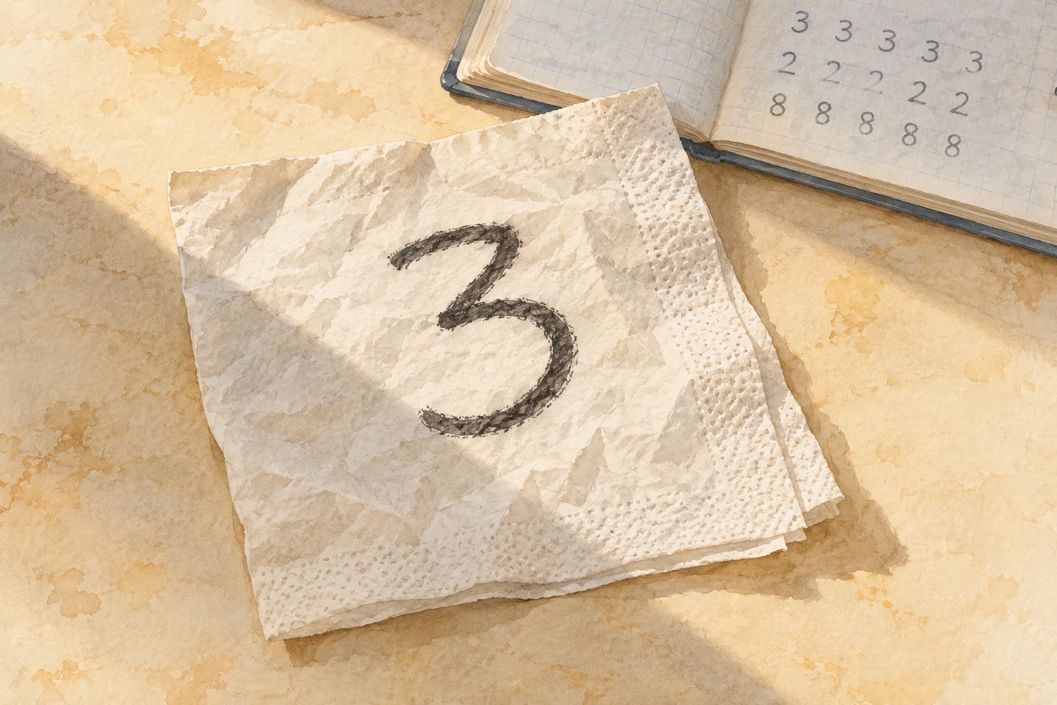
The same 3 under different conditions: the paper, wrinkles and light have changed. A conceptual illustration of the article’s opening scene.

The notebook already contained decisions

For our recognizer, an example can be an image paired with the number it should identify. The image is the input; that number is the label, the reference answer against which we compare the prediction. Collecting many such pairs gives us a dataset. The portion we use to adjust parameters will be the training set.

It sounds straightforward: gather images and record the numbers. Yet someone had to decide who would write, which camera to use, how much space to leave around the digit and what to do with a mark one person reads as 3 and another as 8. Someone also had to check that each crop stayed with its label. A wrong label turns a perfectly legible image into a contradictory learning signal.

Before collecting more, it helps to specify what we want to recognize. Centered digits on a scanned form? Handheld photographs with shadows and folded paper? In the second case, filling the folder with more pages from the same notebook leaves much of the difficulty untouched. We can increase the file count without adding much variety to the situations represented.

We will use representativeness to describe the relationship between the examples collected and the conditions in which we intend to use the model. In our scene, we need variation in handwriting and image capture that matters for that use. Deciding which variation matters requires describing the system’s destination.

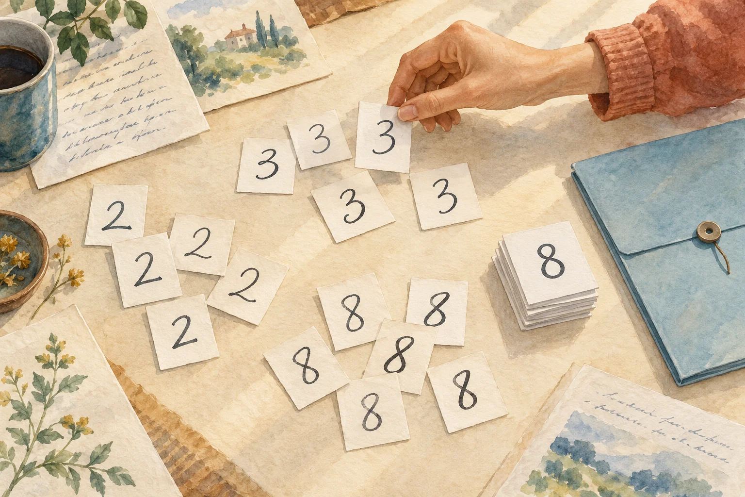
Choosing examples is part of building a model. A conceptual illustration; the cards do not belong to an actual dataset.

When the background helps too much

Suppose that, for convenience, we crop all the 3s from a squared notebook and all the 8s from plain white sheets. We have introduced a clue: the background helps distinguish the labels. If that clue persists in the evaluation examples, a model could exploit it and perform well even if its recognition of the strokes is fragile.

This possibility is studied as shortcut learning: rules that work under the observed conditions and fail when those conditions change. An analysis by Robert Geirhos and coauthors examines this problem in deep networks (Geirhos et al., 2020 (opens in a new tab)).

To investigate, we could keep the same digit and change the background, or compare results across paper types. If predictions changed substantially, we would have a lead to follow. Repeating the comparison and controlling the other changes would help us distinguish the effect of the background from the effect of the test itself.

This difficulty also changes what we mean by quality. If the intended use includes photographs with shadows, removing every shadowy image could leave us with a tidier, less useful collection. We want to remove corrupt files, correct mistaken labels and preserve the difficulty that belongs to the task. The 3 on the napkin should not disappear just because it is less photogenic.

A hundred copies are not a hundred different experiences

While organizing the crops, we discover that one image was saved several times. We might think it merely takes up space. However, if we sample files with equal probability for training, each copy gives that example another opportunity to contribute to parameter updates.

Let us do a small calculation. We start with one hundred distinct images and add ninety-nine copies of one of them. There are now 199 files, one hundred showing exactly the same image. With uniform sampling over files, that image goes from a 1% selection probability to accounting for roughly half of the expected selections. We have changed how often the model encounters that image. Note 1 shows how the repetition appears in an average loss.

Something similar can happen in a text collection when different pages reproduce the same document or share long passages. Deduplication means detecting and handling those repetitions. One example is Colossal Clean Crawled Corpus, a collection of text extracted from the web known as C4 (not the explosive). In their experiments with language models trained on that collection, Katherine Lee and collaborators reduced the proportion of generated tokens belonging to memorized passages to roughly one tenth. They compared models trained on the original corpus and deduplicated versions, generating text without supplying an opening sequence (Lee et al., 2022, section 6.2 (opens in a new tab)).

Nor should we delete everything that looks alike. Two people can write nearly identical 3s and provide independent examples; two pages can contain versions of the same text. We need to decide what counts as a duplicate and at what scale to look for it. Note 2 expands on that distinction. For our notebook, we would start by tracing which crops came from the same capture.

Saving examples for a different question

We now have a more varied collection and know about its repetitions. We still need to decide how to tell whether the model can recognize something it did not use for learning.

Three roles are commonly separated: training, to adjust parameters; validation, to choose configurations during development; and testing, to evaluate the final choice on reserved examples. Repeatedly consulting the test set to make decisions brings it into the development process (scikit-learn developers, n.d. (opens in a new tab)).

In our case, putting files in three folders is not enough. Imagine using a photo of a 3 for training and saving a slightly cropped copy, under a different name, in the test folder. That copy retains almost all the handwriting, background and lighting of the original photo. The model could exploit those similarities to get the answer right while still failing on a 3 written by someone else. The test would then give an overly favorable impression: some of what we present as new was already in training. This is a case of data leakage, because information that should have been reserved for evaluating the model entered its learning process. When that information consists of the evaluation examples themselves, or copies of them, it is called evaluation contamination.

The split should reflect what we want to find out. Crops from one writer share handwriting habits and can be related: treating them as independent observations overlooks that relationship. If we care about recognizing new people’s handwriting, we would hold out entire writers: all crops from each person would go into a single partition. This is why scikit-learn’s evaluation methods keep related groups apart (scikit-learn developers, n.d., section 3.1.2.4 (opens in a new tab)). If we want to measure what happens with another camera, we would also prepare a test that changes that condition.

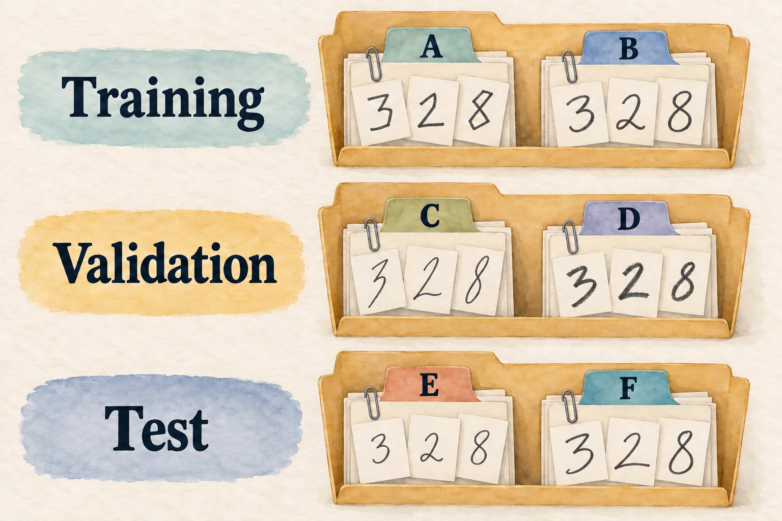
Each letter represents one writer. The digits are the same—3, 2 and 8—but the handwriting changes; all crops from each writer stay in the same partition. This lets us evaluate handwriting from people who were not included in training. The diagram illustrates the grouping rule; partition sizes are a separate decision.

This decision has a precedent in MNIST, a collection of handwritten digits. The US National Institute of Standards and Technology (NIST) had prepared images of handwritten numbers for training and testing, but they came from different populations: the training images came from Census Bureau employees and the test images from high-school students. Yann LeCun and colleagues mixed both sources to construct MNIST and reduce how much results depended on that split. When splitting the images from the 500 students, they assigned the first 250 writers to training and the other 250 to testing (LeCun et al., 1998, section III.A (opens in a new tab)). Where the data came from and who wrote it were already shaping evaluation.

Even with that separation, one percentage can hide precisely what concerns us. Imagine a test of one hundred images: ninety clean and ten with shadows. The model gets all ninety clean images right, but only two of the other ten. That is an overall accuracy—the proportion of correct answers—of 92%, but 20% on images with shadows. If shadows are common in the intended use, the average alone tells an overly comfortable story.

The test also needs enough examples of the conditions we care about. With only ten images, each correct answer moves the result by ten percentage points. Note 3 shows how much uncertainty can accompany that 20%.

From the notebook to a text corpus

Let us take these decisions into language. Instead of crops, we gather documents: articles, manuals, conversations or code, depending on the purpose. An organized collection of texts is called a corpus. The material changes, but we still have to decide what enters, how often it repeats and what to reserve for evaluation.

There is a difference from our labeled digits. For some language training objectives, we can obtain the reference answer from the text itself. In “The fisherman sat on the bank,” for example, we can use a prefix to predict the token that follows, or hide a passage and learn to reconstruct it. Because the reference answer comes from the text itself, this kind of training is called self-supervised learning. The work by Colin Raffel and coauthors compares objectives of this kind under the name “unsupervised objectives” (Raffel et al., 2020, section 3.3 (opens in a new tab)). Words make the example easier to read; processing uses tokens, which do not always correspond to whole words.

The text supplies a reference for that task, but the reference does not certify the truth of what was written. A mistaken sentence also has a next token. We can prepare examples for learning regularities in language without having verified every claim in the corpus. That distinction will matter when we ask what it means for a model to know something; for now, it explains why the material’s origin matters before training begins.

Following a document from its source makes those decisions concrete. Imagine a page explaining something about fishing. Extracting it might bring along the menu, a repeated notice and recommendations for other articles. We would then need to identify the language, check whether the content is complete, detect copies and decide where it belongs in our collection. Each transformation should leave enough of a trail to tell what we kept and what we lost.

The C4 corpus offers a documented case: its authors began with text extracted from the web and applied filtering rules (Raffel et al., 2020, section 2.2 (opens in a new tab)). Naming a data source tells only part of its story; the rules applied afterward also determine the material that reaches training.

What a filter leaves out

We can see this on our imagined page. A rule that removes repeated menus seems reasonable; one that discards short texts could also remove a concise, valuable explanation. If we always favor a formal register, we could reduce the presence of the everyday language we later expect the model to handle.

A study of C4 by Jesse Dodge and other researchers found that filtering with a blocklist of words disproportionately removed text by and about people belonging to minority groups (Dodge et al., 2021, sections 5.2–5.3 (opens in a new tab)).

For our fishing collection, we would therefore inspect both the accepted material and a sample of what was rejected. Are we losing vocabulary from a particular region? Does the language detector discard pages that mix Spanish and English? Even the “Clean” in Colossal Clean Crawled Corpus needs that inspection to give it meaning.

A filter can also let through material we meant to hold apart. That same study detected examples from evaluation datasets inside C4 (Dodge et al., 2021, section 4.2 (opens in a new tab)). This is the contamination we saw in the notebook, now at web scale: some of the material reserved for evaluation was already among the documents available for training.

Deduplication also reaches across that boundary between folders. Lee’s deduplication study also found, using its method for detecting near-duplicate documents, that 4.6% of C4 validation examples had an approximate duplicate in training (Lee et al., 2022, table 2 (opens in a new tab)). Comparing the partitions with each other helps locate the textual equivalent of that crop saved in two folders.

We would also decide how often to present each source. Suppose that, after filtering, we have 900 manuals and 100 conversations. If we sample documents uniformly with replacement—a document can be selected again—conversations account for 10% of expected selections. If we choose the source first and reserve 30% for conversations, we expect about 300 conversation selections out of 1 000, instead of 100. We still sample uniformly within that source: each of the same one hundred conversations appears three times on average instead of once. That leaves 700 selections for the 900 manuals: each goes from one expected appearance to about 0.78 (700/900). We have increased exposure to conversations at the expense of manuals, while keeping one hundred distinct conversations. This is the difference between getting other notebooks and photocopying the first one.

A collection we can explain

By this point, the folder of images or documents comes with a history: where it came from, what we selected, how we resolved ambiguities and what we left out. Someone receiving only the files would have to guess much of it.

The datasheets for datasets proposal, presented by Timnit Gebru together with other researchers, aims to document a collection’s motivation, composition, collection process, preprocessing—including cleaning and labeling—uses, distribution and maintenance (Gebru et al., 2021 (opens in a new tab); accessible manuscript (opens in a new tab)).

Applied to our project, that framework would let us reconstruct which people and conditions supplied the digits, what permissions were recorded, how labels were assigned and which versions ended up in each partition. For the corpus, we would add the sources, documented conditions of use and transformations applied. When something is unknown, stating that explicitly preserves a question that would otherwise remain hidden.

That traceability helps us investigate the next error. If the model fails on a photo, we can ask whether the condition was represented, whether processing altered a stroke or whether our evaluation already pointed to the difficulty. The datasheet gives us concrete places to look.

Back to the 3 on the napkin

The opening scene is unchanged: a person sees a 3 and the computer gets it wrong. Now we have a way to investigate that possible distribution shift. We can examine the training examples, accidental clues, repetitions and how the test was constructed. Perhaps we need different images; perhaps the problem is in the cropping or the model. We know what to compare to begin distinguishing those possibilities.

We can also look differently at a claim such as “it was trained on enormous amounts of data.” We will want to know which data, selected by what criteria, repeated how often and evaluated against which situations. Those questions give substance to a claim that, on its own, told us very little.

We have prepared the material and the conditions for assessing learning. The next step will be to follow how a language model uses that material to make predictions and adjust its parameters. Before that calculation came something very human: someone decided which examples belonged and what doing well would mean.

Notes

1. Repetition inside the average. For an objective that weights each file’s loss equally, let $\ell_1,\ldots,\ell_{100}$ be the losses of our one hundred images, evaluated with the same parameters. Before copying, the average is:

   $$L=\frac{1}{100}\sum_{i=1}^{100}\ell_i$$

   Adding 99 copies of the first image changes it to:

   $$L'=\frac{100\ell_1+\sum_{i=2}^{100}\ell_i}{199}$$

   The coefficient of $\ell_1$ rises from $1/100$ to $100/199$, about 50.3% of the total weight: the same half we found by counting files. This assumes exact copies, equal weighting and the same processing; different sampling changes the calculation. It also does not imply that repeating an entire collection over several epochs has the same effect as multiplying only one example. Return to the copies.

2. Exact and near duplicates. Comparing content hashes helps locate exact copies; finding variants requires similarity criteria. Lee’s paper examines both near-duplicate documents using MinHash and repeated substrings using a structure called a suffix array (Lee et al., 2022, section 4 (opens in a new tab)). The threshold and unit of comparison matter: removing a duplicate page is different from removing a shared passage. Return to deduplication.

3. The uncertainty in ten images. If the ten images were independent observations from the same population and each prediction had the same probability of success, 2 correct answers out of 10 would give a 95% exact Clopper–Pearson binomial interval of approximately 2.5% to 55.6%. The method comes from Clopper and Pearson (1934) (opens in a new tab); SciPy developers (n.d.) (opens in a new tab) document an implementation. That interval shows how imprecise the estimate is with such a small sample. The 95% describes the procedure’s coverage over repeated sampling; it does not assign a probability to the parameter after observing the data. If several images share a writer or capture, we must account for that dependence when estimating uncertainty. Return to evaluation.

References

Clopper, C. J., & Pearson, E. S. (1934). The use of confidence or fiducial limits illustrated in the case of the binomial. Biometrika, 26(4), 404–413. https://doi.org/10.1093/biomet/26.4.404 (opens in a new tab)

Dodge, J., Sap, M., Marasović, A., Agnew, W., Ilharco, G., Groeneveld, D., Mitchell, M., & Gardner, M. (2021). Documenting large webtext corpora: A case study on the Colossal Clean Crawled Corpus. In M.-F. Moens, X. Huang, L. Specia, & S. W.-t. Yih (Eds.), Proceedings of the 2021 Conference on Empirical Methods in Natural Language Processing (pp. 1286–1305). Association for Computational Linguistics. https://doi.org/10.18653/v1/2021.emnlp-main.98 (opens in a new tab)

Gebru, T., Morgenstern, J., Vecchione, B., Vaughan, J. W., Wallach, H., Daumé, H., III, & Crawford, K. (2021). Datasheets for datasets. Communications of the ACM, 64(12), 86–92. https://doi.org/10.1145/3458723 (opens in a new tab). Authors’ manuscript (opens in a new tab)

Geirhos, R., Jacobsen, J.-H., Michaelis, C., Zemel, R., Brendel, W., Bethge, M., & Wichmann, F. A. (2020). Shortcut learning in deep neural networks. Nature Machine Intelligence, 2(11), 665–673. https://doi.org/10.1038/s42256-020-00257-z (opens in a new tab). Authors’ preprint (opens in a new tab)

LeCun, Y., Bottou, L., Bengio, Y., & Haffner, P. (1998). Gradient-based learning applied to document recognition. Proceedings of the IEEE, 86(11), 2278–2324. https://doi.org/10.1109/5.726791 (opens in a new tab). Authors’ copy (opens in a new tab)

Lee, K., Ippolito, D., Nystrom, A., Zhang, C., Eck, D., Callison-Burch, C., & Carlini, N. (2022). Deduplicating training data makes language models better. In S. Muresan, P. Nakov, & A. Villavicencio (Eds.), Proceedings of the 60th Annual Meeting of the Association for Computational Linguistics (Volume 1: Long Papers) (pp. 8424–8445). Association for Computational Linguistics. https://doi.org/10.18653/v1/2022.acl-long.577 (opens in a new tab)

Raffel, C., Shazeer, N., Roberts, A., Lee, K., Narang, S., Matena, M., Zhou, Y., Li, W., & Liu, P. J. (2020). Exploring the limits of transfer learning with a unified text-to-text transformer. Journal of Machine Learning Research, 21(140), 1–67. Original article (opens in a new tab)

scikit-learn developers. (n.d.). Cross-validation: Evaluating estimator performance. scikit-learn. Retrieved October 4, 2026, from the project documentation (opens in a new tab).

SciPy developers. (n.d.). BinomTestResult.proportion_ci. SciPy v1.16.1 manual. Retrieved October 4, 2026, from the project documentation (opens in a new tab).

People mentioned

Robert Geirhos

Researcher in the behavior and generalization of neural networks. His collaborative work on shortcut learning examines how models exploit patterns that work on familiar data but fail when conditions change.

Sources

• Shortcut Learning in Deep Neural Networks (2020) (opens in a new tab)

Katherine Lee

Researcher in training data for language models. She coauthored a study showing how deduplicating text collections could reduce memorized output and overlap between training and evaluation data.

Sources

• Deduplicating Training Data Makes Language Models Better (2022) (opens in a new tab)

Yann LeCun

Researcher in machine learning and computer vision, known for his work on convolutional neural networks. His research on handwritten digit recognition includes LeNet and the MNIST dataset, which connects model design with the preparation of training and test examples.

Sources

• Yann LeCun — Learning and Visual Perception (opens in a new tab)

Colin Raffel

Researcher in transfer learning for language models. He coauthored the T5 study, which compared training approaches within a text-to-text framework and introduced the C4 text collection.

Sources

• Exploring the Limits of Transfer Learning with a Unified Text-to-Text Transformer (2020) (opens in a new tab)

Jesse Dodge

Researcher in language-model datasets and their documentation. His collaborative analysis of C4 examined the effects of filtering web text and the presence of evaluation examples in training data.

Sources

• Documenting Large Webtext Corpora: A Case Study on the Colossal Clean Crawled Corpus (2021) (opens in a new tab)

Timnit Gebru

Researcher in machine learning and the documentation of its datasets. She coauthored Datasheets for Datasets, a proposal to record a collection’s motivation, composition, collection process and intended uses so that others can assess its suitability.

Sources

• Datasheets for Datasets (2021) (opens in a new tab)