What is a neural network?

Write a 3 on a sheet of paper. Now write another, slightly tilted, and a third with its upper curve almost closed. To you, they are still threes. If you had to tell a computer how to recognize them, what rules would you write? “Look for two curves” sounds like a reasonable start, until a letter with two curves or a poorly closed 8 comes along. Something we recognize easily can be difficult to turn into precise instructions.

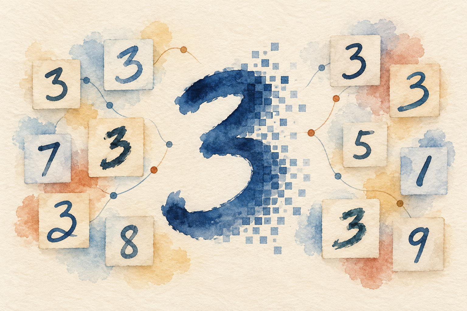
From strokes to pixels: a conceptual illustration inspired by the handwritten digits of MNIST.

An artificial neural network is a mathematical model that connects computational units to transform an input into an output. Its connections have adjustable parameters: by training it with data and an objective, we can change those parameters to produce more useful answers. In our example, the input will be an image and the output an estimate of which digit it contains. The network will learn a way to carry out that transformation, including intermediate representations of the image (Goodfellow et al., 2016, chap. 6 (opens in a new tab)).

In Is AI really new?, we explored some of the ideas that made machine learning possible. Here we will open one of them up. We can follow that 3 from pixels to an answer and, when the answer is wrong, see what correcting the network actually means.

Inside an artificial neuron

To recognize our 3, the computer will receive numbers describing the image. Before considering the whole network, imagine a unit that receives just two of those numbers. An artificial neuron combines its inputs and passes a result to other units. The name retains the biological inspiration of receiving and transmitting signals; here, we can follow every step as a mathematical operation.

The first decision is how much each input contributes. That is what a weight does: it is a number that multiplies the value arriving along a connection. Imagine a volume control for each input, with one important difference: a negative weight makes its contribution subtract from the total. If an input is 0.8 and its weight is 0.5, it contributes 0.4 to the sum. With a weight of 0.1, that same input would contribute 0.08. The image would be identical; what changes is how that unit processes it.

The neuron adds these contributions and includes a bias, another adjustable number that shifts the total. It then needs a rule for determining what value to pass to the next stage. That rule is the activation function: it receives the sum and transforms it. The value it returns is called the neuron's activation.

One common choice is ReLU, short for rectified linear unit. Its rule is simple: if the sum is zero or negative, return 0; if it is positive, return that same amount. A sum of −0.2 becomes 0; a sum of 0.42 passes through as 0.42. It resembles a gate that blocks values on one side of zero and passes those on the other, preserving their strength. It can therefore convey how strongly a unit activated, rather than restricting it to “on” or “off” (Zhang et al., 2023, sec. 5.1.2 (opens in a new tab)).

Why introduce this step? Consider two dark regions of our drawing: their usefulness depends on how they appear together. Weights and the bias allow one combination of inputs to produce a positive sum while another stays at or below zero; ReLU passes a response in the first case and zero in the second. Combining many such units lets the network respond differently to different combinations of pixels. ReLU's rule is fixed in this example; training changes the weights and biases that determine which inputs activate it.

The formula can now summarize something we already understand. With inputs $x_1$ and $x_2$, weights $w_1$ and $w_2$, bias $b$ and activation $g$:

The first line calculates the sum $z$; the second produces the response $a$ that other units will receive. For ReLU, $g(z)=\max(0,z)$ means choosing the larger of zero and the sum. The bias also has a practical effect: shifting $z$ changes which combinations of inputs cross zero. Weights and biases are parameters, the model's adjustable numbers.

Let us calculate an example using illustrative values. With inputs of 0.8 and 0.2, weights of 0.5 and −0.4, and a bias of 0.1:

Changing only the first weight from 0.5 to 0.7 raises the response from 0.42 to 0.58. The same inputs now produce a stronger signal for the next unit. That is the concrete effect of adjusting a weight; whether it helps recognize the 3 will depend on the network's final answer. First, we need to connect this small operation to the others.

From pixels to a representation

Our 3 occupies many points in the image, so let us expand the example. Prepare a grayscale image of $28\times28$ pixels: a grid of 784 positions. At each position, write a number between 0 and 1; for this example, 0 represents the white background and 1 the black ink, with intermediate values for shades of gray. We have turned the drawing into 784 numbers the network can process. Those numbers form the input.

We will design a simple network with one layer of 64 neurons and an output of ten values, one for each digit from 0 to 9. Each neuron in that layer receives all 784 values, with its own weights and bias. Their 64 responses pass to the output units. We choose 64 to make the architecture concrete. The right size for an actual model would depend on the task and experimental evaluation.

Where are the weights defined? When these layers are built, the program creates tables of numbers—matrices—with a weight for each connection and a bias for each neuron. The network designer chooses the connections and how to initialize those numbers; when training from scratch, weights usually begin with random values at an appropriate scale. The training algorithm then adjusts them. We do not have to write the correct weight for each stroke by hand. The same set of weights is used for all images passing through the network; that ability to reuse an adjustment is what we want to exploit (Goodfellow et al., 2016, sec. 8.4 (opens in a new tab); Zhang et al., 2023, sec. 6.2 (opens in a new tab)).

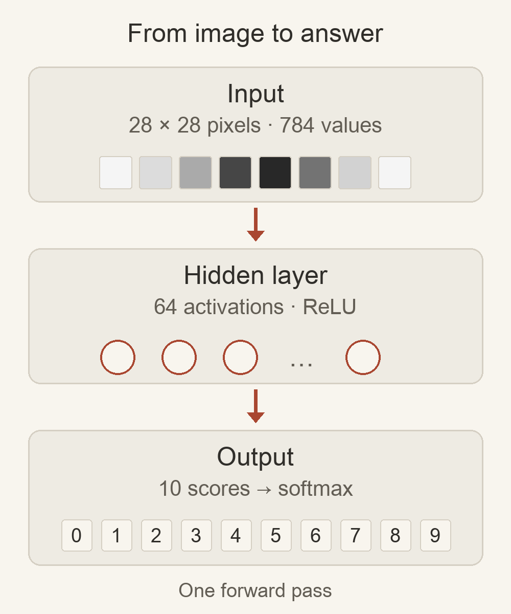
One possible network for our example. Each block represents a stage of computation; individual connections are omitted. The sizes describe an illustrative design.

The intermediate layer is called hidden because it sits between the input and the final answer; its values can be calculated and inspected. Consider what just happened: we went from describing where the ink is with 784 numbers to describing the responses of 64 units. That new list is a representation of the image. If those responses distinguish useful combinations of strokes, the next stage has a better basis for separating a 3 from an 8. Training adjusts how that representation is built using the final answer, without needing a correct label for each hidden neuron (Rumelhart et al., 1986 (opens in a new tab)).

It is tempting to imagine one neuron detecting “upper curve” and another detecting “lower curve.” That can help us picture the idea, but it is not a guaranteed description of what our network will learn. A feature can depend on many units, and the same unit can participate in several distinctions.

We can add layers to combine those responses again. That composition is central to deep learning. Here we can see why activation mattered: if every stage only multiplied and added, the entire chain could be summarized by one operation of the same kind, an affine transformation. ReLU introduces a change in behavior at zero: different inputs activate different sets of units. This nonlinearity allows layers to build more complex relationships instead of merely recalculating a longer sum (Goodfellow et al., 2016, secs. 6.1–6.4 (opens in a new tab)). We now have a structure that can transform the drawing; let us follow one image all the way to its answer.

The forward pass: producing an answer

Give the network the image of our 3. It first calculates the 64 hidden activations using its current weights. It then uses them to calculate ten output scores: one for 0, another for 1, and so on up to 9. Each score combines responses from the previous layer with another set of weights. This is forward propagation, or the forward pass. Because the connections run from input to output without forming cycles, we call this a feedforward architecture.

The final scores, also called logits, let us rank the options. If the score for 8 is highest, our decision rule will select that class, even though we see a 3. But “8 has the highest score” leaves a useful question open: is it far ahead of the others, or almost tied with 3?

To express how the prediction is distributed across the options, we use softmax. This function transforms the ten scores into positive probabilities that sum to 1. Imagine a total of 100% divided among ten boxes: higher scores receive a larger share. The formula uses exponentials to obtain positive values and divides each by their total; this preserves the ranking and puts the outputs on a common scale (Zhang et al., 2023, sec. 4.1 (opens in a new tab)).

Softmax fits this task because each image has one correct label among ten alternatives. If we only wanted to choose the highest score, we could do that directly. The distribution adds something we will use when learning: it distinguishes a prediction that assigns little probability to 3 from one that assigns it a lot, even when both choose the same class. It also changes smoothly as the scores change, which will let us calculate how to adjust the weights. Note 1 brings together the formula and the notation for the complete network.

For example, 0.8 for digit 3 means the model assigns it 80% of the probability among those options. Whether it is right 80% of the time in similar situations needs to be checked against data: that correspondence is called calibration (Guo et al., 2017 (opens in a new tab)). And if we show it a letter, softmax will still distribute probability among digits, because those are the only options we designed. The distribution describes the model's output within that task.

We have an answer, but we are still using the weights we started with. Learning will mean changing those parameters using examples and a measure of error, seeking more useful answers. Repeating this pass with the same image and parameters in our network would give us the same result. To move forward, we need something the calculation alone cannot provide: a way to evaluate the answer.

Giving the error a measure

For our 3, we know the correct answer. During training, we provide it to the system alongside the image, and do the same with examples of the other digits. This is supervised learning. The label serves as the answer to an exercise: it lets us correct the attempt. When we later show a new image for recognition, the model will have to answer using its learned parameters.

But correcting an answer only with “right” or “wrong” would provide a limited signal. If the network raises its probability for 3 from 0.2 to 0.3 while still choosing 8, it has moved in a useful direction for that example even though it remains wrong. A loss function turns the difference between prediction and target into a number that can reflect this progress. For our classifier, we use cross-entropy: when the correct label is 3, it gives a higher loss if the model assigns it little probability and a lower loss if it assigns it a lot. We write it as:

Here $p_3$ is the probability assigned to the correct digit, and we use the natural logarithm. If $p_3=0.2$, the loss is approximately 1.61; if $p_3=0.8$, it is approximately 0.22. The rule rewards assigning more probability to the correct answer, even when the winning class was already right. Counting correct answers and measuring loss are different ways to evaluate behavior (Zhang et al., 2023, sec. 4.1 (opens in a new tab)).

We usually group several examples into a batch and calculate an average loss to guide an adjustment. The question becomes more than “was it wrong?” We now ask how its parameters would need to change to reduce that loss.

The learning signal depends on the task. In self-supervised learning, for instance, the target can be constructed from the data themselves, by hiding a part and asking the model to predict it. We still need a task and a loss; a person does not have to write a label for every example. Predicting hidden parts of a text is one example of this approach (Zhang et al., 2023, sec. 15.8 (opens in a new tab)). This distinction will matter when we move from images to language.

Return to our digit: the label gives us a target, softmax gives us a distribution, and the loss tells us how far the prediction is from that target under our chosen measure. What we still need is a way to connect that final number to each adjustable weight.

Backpropagation: connecting the error to the parameters

Remember the weight we changed from 0.5 to 0.7: it raised one neuron's response from 0.42 to 0.58. We now need to know whether that increase helps recognize the 3 or reinforces a wrong answer. That depends on what later units do with the signal. The loss is at the end of the path, but the weight had an influence much earlier: it changed an activation, which changed the scores, which changed the probabilities. We need to follow that chain of dependencies.

Backpropagation calculates how the loss varies locally with respect to each parameter. It traverses the operations in reverse and applies the chain rule, which combines derivatives of connected operations. It reuses intermediate results, so it does not need to test each weight separately to estimate its effect (Zhang et al., 2023, sec. 5.3 (opens in a new tab)).

In practical terms, we want to know: “If I nudged this volume control upward, would the loss rise or fall? By how much?” A derivative expresses that local sensitivity, and the collection of derivatives with respect to the parameters forms the gradient. Backpropagation calculates those answers efficiently by following the network's operations. Note 2 works through a complete numerical example.

An optimizer then uses those gradients to change the parameters. A simple gradient-descent update is:

The arrow means “replace the old value.” The symbol $\eta$ is the learning rate, which controls the size of the step. If the derivative is positive, the rule decreases the weight; if it is negative, it increases it. Backpropagation computes the gradient, and the optimizer determines the adjustment. These are distinct parts of the process.

The learning rate is how far we turn each control after receiving that guidance. A very small step may make progress slow; a very large one can overshoot and make the loss worse. For our image, the adjustment changes how the pixels contribute to hidden responses and how those responses contribute to the ten scores. A later pass can therefore assign the 3 a different probability even though the image itself has not changed.

With the new parameters, we repeat the forward pass on another batch. An epoch is a complete pass through the training dataset. Predict, measure loss, compute gradients and update: that cycle gives “the network learns” a concrete meaning. Step size and the shape of the problem affect that search: an update can help some examples and hurt others, and training can settle on a solution that is not the best possible one (Goodfellow et al., 2016, chap. 8 (opens in a new tab)).

This also explains one difficulty of stacking many layers. Backpropagation combines sensitivity factors along the path. Those products can become extremely small, leaving some weights with barely any adjustment, or extremely large, making updates unstable. These are vanishing and exploding gradients, difficulties in optimization, the search for parameters that reduce the loss. Initialization and network design help make depth usable (Goodfellow et al., 2016, secs. 8.2.4–8.2.5 and 8.4 (opens in a new tab)).

We can now say what learning means in this model: examples guide changes to numbers that will be reused on later inputs. We can save those parameters and load them to run the network again (Zhang et al., 2023, sec. 6.2 (opens in a new tab)). The practical question becomes whether those adjustments also help with a 3 written by someone else.

Recognizing a three it has never seen

Let us try that other 3. If all the training examples came from the same notebook, perhaps the network used details of the background that disappear on the new page. It may have reduced the loss and still fail now. That is the practical difference between improving on familiar exercises and being able to solve one we had not shown it.

We want generalization: useful behavior that holds for examples not used for training. We set aside validation data to guide decisions, such as when to stop training, and a test set to evaluate the final result. If we continually used the test set to choose changes, it would cease to be an independent evaluation. Overfitting occurs when the model adapts too closely to its training examples and performs worse on others (Goodfellow et al., 2016, sec. 5.2 (opens in a new tab)).

Once the network is trained, we can give it another 3 and run inference: using the learned parameters to produce an answer. Activations will change with each image, while weights remain fixed in this ordinary use. For this classifier, that means using the forward pass to recognize the new image.

This separates two things we sometimes mix together when discussing learning: a different response to a different input, and a lasting change in the parameters. If we later want to adapt the model using new data, we will need another training process. And if those data come from different conditions, we will need to check its behavior again.

Different networks for different structures

Suppose the new 3 is also shifted to one side of the image. We still recognize its shape, but the ink now occupies different input positions. This gives us a reason to revisit how we arranged the connections. Our example connects every input to every neuron in the next layer. It uses dense layers and is also called a multilayer perceptron, or MLP. It helps us understand the mechanism, but flattening the image into a list does not explicitly build in the fact that some pixels are neighbors. The architecture determines what connects to what, which operations are performed and which parameters are shared. We can choose designs that make better use of the problem's structure.

Convolutional neural networks, or CNNs, apply learned filters to local regions, reusing their weights at different positions. A filter that responds to a particular stroke can therefore be applied in different parts of the image. Successive layers combine information from increasingly large regions. For our digit, this builds in a useful idea: a stroke remains relevant even if it moves a little. This introduces spatial structure into the model; how well it handles shifts still depends on the complete architecture and training (Zhang et al., 2023, sec. 7.1 (opens in a new tab)).

The structure of the input can change in another way. Imagine recording the pen movements as someone draws the 3: we now receive a sequence whose order matters. Recurrent neural networks, or RNNs, process sequences while maintaining a state that is updated at each step. On receiving a new element, they use both that element and information from the previous state. LSTM is a variant with mechanisms that regulate the flow and retention of information, designed to make long-range dependencies easier to learn. What persists in that state depends on the learned updates and gates (Hochreiter & Schmidhuber, 1997 (opens in a new tab)).

For sequences, we can also design a mechanism that combines information from other positions directly. Transformers combine attention mechanisms, which weight information from different positions, with feedforward network blocks and other operations. Attention lets a representation incorporate context from other parts of the input. In a causal variant, positions cannot consult future elements. For now, the idea to keep is that how information is related is also part of a network's design (Vaswani et al., 2017 (opens in a new tab)).

These families illustrate different choices about connections and computation, and those choices can coexist in one model. A CNN can be feedforward; a Transformer contains feedforward blocks. Their usefulness depends on the task and the structure of the data.

How networks can work together

Now imagine a photograph containing several digits. We could design a system in which one component locates each symbol and another recognizes the cropped images. We could also build a network that transforms the whole image into a sequence of digits. These are two possible ways to divide the work; they require different training arrangements and interfaces between components.

A common combination is an encoder–decoder: one network transforms the input into a representation, and another uses that representation to produce the output. Cho and colleagues studied this arrangement with recurrent networks to relate word sequences in translation (Cho et al., 2014 (opens in a new tab)). “Encoder” and “decoder” name roles within a system; different architectures can fill them.

When components are trained together and the path supports gradient propagation, a final loss can guide adjustments throughout them. If we train them separately or keep one fixed, adaptation will work differently. We can also combine several networks' predictions in an ensemble, without making them a single network trained end to end.

So when we say networks “interact,” it helps to look at what they exchange: activations, representations, probabilities or results that another program turns into inputs. The system we build defines that connection: the output of one calculation becomes material for the next.

What this contributes to artificial intelligence

Return to the 3 on the paper. At first, it seemed we needed a rule for every variation in handwriting. A neural network offers another possibility: designing a computational process whose parameters and representations can be adjusted from examples. We still choose data, architecture, objectives and evaluation criteria, but an important part of how to transform the input is learned during training.

That is one of its contributions to AI: learning useful representations for recognizing, predicting or generating, in tasks where spelling out every pattern by hand is difficult. The same general framework accommodates different outputs: a category, a quantity or a distribution from which to generate elements of a sequence. AI also includes other methods, and a neural network may be just one component of an application.

A language model takes the problem toward sequences of text. To reach an LLM, or large language model, we will need to explore how to represent that text, how to relate its parts, and which objectives and scale to use in training. The Transformer is one architecture that can be used along that path; not every Transformer is an LLM, and not every neural network works with language.

An agentic system adds another arrangement: it uses a model within a loop that can choose actions, consult tools and process their results. Work such as ReAct studies how to interleave the model's generation with actions in an environment (Yao et al., 2023 (opens in a new tab)). Understanding that system requires looking at both the network and the program that puts it to work.

Our 3 is still a 3, but we can now describe what happens when we show it to the machine. Pixels become activations, activations become a prediction and, during training, the loss guides changes to the parameters. That distinction between representing, computing and learning will let us move toward more complex systems while keeping track of what each part does.

Notes

1. The network in compact notation. We can write the hidden layer as $\mathbf{h}=\operatorname{ReLU}(W_1\mathbf{x}+\mathbf{b}_1)$ and the output scores as $\mathbf{s}=W_2\mathbf{h}+\mathbf{b}_2$. Bold letters represent lists of numbers, or vectors; the matrices $W_1$ and $W_2$ collect the weights. In our design, their shapes are $64\times784$ and $10\times64$. For each digit $k$, softmax computes $p_k=\frac{e^{s_k}}{\sum_{j=0}^{9}e^{s_j}}$. Exponentials are positive, and dividing them by their sum makes the probabilities sum to 1. The formula describes the mathematical result; implementations use a numerically stable version. See Zhang et al. (2023, sec. 4.1) (opens in a new tab). Return to the forward pass.

2. An update we can check. Isolate a scalar model $\hat{y}=wx$ with loss $L=\frac{1}{2}(\hat{y}-y)^2$. This is an arithmetic example, not our digit classifier. The chain rule gives $\frac{\partial L}{\partial w}=(\hat{y}-y)x$. With $x=2$, $y=1$ and $w=0.2$, the prediction is 0.4, the loss is 0.18 and the gradient is −1.2. If $\eta=0.1$, the new weight is $0.2-0.1(-1.2)=0.32$. The new prediction is 0.64 and the loss falls to 0.0648. In a network, the same rule applies to longer chains and adds contributions when there are multiple paths. The size of the step matters: an excessive learning rate can increase the loss. ReLU also has no unique derivative at zero; implementations use a convention at that point. Return to backpropagation.

References

Cho, K., van Merriënboer, B., Gulcehre, C., Bahdanau, D., Bougares, F., Schwenk, H., & Bengio, Y. (2014). Learning phrase representations using RNN encoder–decoder for statistical machine translation. In A. Moschitti, B. Pang, & W. Daelemans (Eds.), Proceedings of the 2014 Conference on Empirical Methods in Natural Language Processing (EMNLP) (pp. 1724–1734). Association for Computational Linguistics. https://doi.org/10.3115/v1/D14-1179 (opens in a new tab)

Goodfellow, I., Bengio, Y., & Courville, A. (2016). Deep learning. MIT Press. Chapter 5: Machine learning basics (opens in a new tab). Chapter 6: Deep feedforward networks (opens in a new tab). Chapter 8: Optimization for training deep models (opens in a new tab)

Guo, C., Pleiss, G., Sun, Y., & Weinberger, K. Q. (2017). On calibration of modern neural networks. In D. Precup & Y. W. Teh (Eds.), Proceedings of the 34th International Conference on Machine Learning (Vol. 70, pp. 1321–1330). PMLR. Conference proceedings (opens in a new tab)

Hochreiter, S., & Schmidhuber, J. (1997). Long short-term memory. Neural Computation, 9(8), 1735–1780. https://doi.org/10.1162/neco.1997.9.8.1735 (opens in a new tab)

Rumelhart, D. E., Hinton, G. E., & Williams, R. J. (1986). Learning representations by back-propagating errors. Nature, 323, 533–536. https://doi.org/10.1038/323533a0 (opens in a new tab)

Vaswani, A., Shazeer, N., Parmar, N., Uszkoreit, J., Jones, L., Gomez, A. N., Kaiser, Ł., & Polosukhin, I. (2017). Attention is all you need. In I. Guyon, U. von Luxburg, S. Bengio, H. Wallach, R. Fergus, S. V. N. Vishwanathan, & R. Garnett (Eds.), Advances in Neural Information Processing Systems (Vol. 30, pp. 5998–6008). Curran Associates. Conference proceedings (opens in a new tab)

Yao, S., Zhao, J., Yu, D., Du, N., Shafran, I., Narasimhan, K., & Cao, Y. (2023). ReAct: Synergizing reasoning and acting in language models. In The Eleventh International Conference on Learning Representations. Conference paper — OpenReview (opens in a new tab). Preprint — arXiv, v3 (opens in a new tab)

Zhang, A., Lipton, Z. C., Li, M., & Smola, A. J. (2023). Dive into deep learning. Cambridge University Press. Book and cited chapters (opens in a new tab)