From words to vectors: tokens, embeddings and why meaning becomes geometry

Imagine reading “The bank flooded after the storm.” Perhaps you picture a river overflowing. Perhaps you picture water coming through the doors of a bank branch. The sentence gives us clues, but it leaves room for both readings. Even a familiar word needs company before we can decide what it means here.

One word, two possible meanings: a conceptual illustration of the journey from language to geometric representations.

A language model faces an earlier problem: how does that sentence become something a neural network can calculate with? In the previous article, we followed a network from its input to a prediction and saw how errors guide learning. This time, the input is language. Before any layer can work with it, the text needs a numerical representation.

Following that transformation will take us through three things that are easy to confuse: tokens, identifiers and embeddings. We will keep the same sentence in view. By the time we return to its ambiguity, we will be able to explain what those three steps contribute—and what still remains to be done.

First, decide where to cut

We usually read the sentence as words separated by spaces. A tokenizer, the component that prepares text for the model, works with a vocabulary of pieces called tokens. A piece might be a whole word, part of a word, punctuation or a sequence that includes a space.

Suppose our tokenizer produces the following pieces. This is an invented example, not the output of a particular system:

[The] [ bank] [ flooded] [ after] [ the] [ storm] [.]

The spaces inside the brackets are intentional. This convention appears in tokenizers such as GPT-2’s, whose preprocessing can group a leading space with the following letters before applying byte-level BPE (OpenAI, 2019 (opens in a new tab)). Our pieces and IDs remain illustrative. With another vocabulary, riverbank might stay whole or split into river and bank. These boundaries reflect the tokenizer’s rules, rather than a grammar lesson.

Why go to that trouble? Keeping one token for every possible word would mean accounting for names, spelling variants and words we have not encountered yet. Characters offer smaller reusable pieces, but turn even a short phrase into a longer sequence. Subword tokenization makes room between those choices: frequent sequences can stay together, while rarer words can be assembled from smaller units.

One influential method is byte-pair encoding, or BPE. In its adaptation for translation, it starts with characters and repeatedly merges the most frequent adjacent pair of symbols. The resulting pieces can participate in later merges, building a vocabulary of variable-length units (Sennrich et al., 2016, section 3.2 (opens in a new tab)). Training the tokenizer learns those rules; using it applies them to new text.

Different tokenizers make different choices about their starting symbols and rules. “Subword” alone does not guarantee coverage of every possible input; note 1 explains that qualification. For our sentence, the immediate consequence is concrete: the chosen boundaries determine how many pieces the network will process and which pieces can reuse the same initial representation.

A number that tells us where to look

Once the pieces are chosen, each has an integer identifier in the vocabulary. Let us give our invented tokens invented IDs:

Token	Illustrative ID
The	104
bank	7312
flooded	29041
after	889
the	262
storm	5774
.	13

Notice The and the: capitalization and the leading space make them different pieces, so our vocabulary assigns them different IDs. The sentence is now the sequence [104, 7312, 29041, 889, 262, 5774, 13]. We have numbers, but they tell us which pieces were selected. Subtracting 7312 from 29041 would reveal nothing about the relationship between a bank and a flood. The integers function as addresses, much like row numbers in a table.

We could also express each address as a one-hot vector: a list with a 1 at that token's position and 0 everywhere else. That distinguishes every token. Multiplying coordinates in matching positions and adding the products—the dot product—gives zero for any two different one-hot vectors. Geometrically, they are perpendicular, or orthogonal. The representation itself gives us no graded similarity. A model can still learn from those inputs; it needs learned parameters to establish useful relationships between them. The connection to the lookup we are about to use is in note 2.

The address gives us a way to retrieve the learned information associated with that token.

The row behind the address

Picture a table with one row for each token and the same number of numerical columns in every row. That is the embedding table. The ID selects a row, and the row supplies a vector: an ordered list of values that the network can work with.

For illustration, suppose the row at address 7312 contains just three values:

Looking up bank retrieves that list. We have not calculated the three values from the digits in 7312; they were stored in the selected row. Both the ID and the values here are invented. Three dimensions keep the example readable, while a real model may use hundreds or thousands.

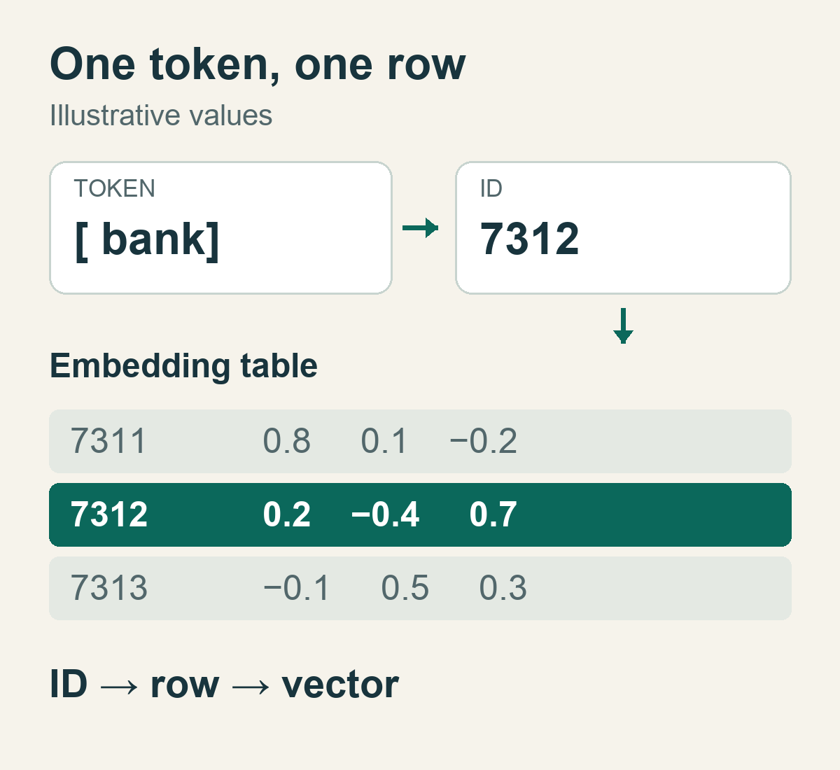
An illustrative lookup: the identifier selects a row; the row supplies the vector. These are invented values, not measurements from a trained model.

If the vocabulary contains $|V|$ tokens and each vector has $d$ values, the whole table is a matrix $E \in \mathbb{R}^{|V| \times d}$. For the token at sentence position $j$, whose ID is $i_j$, the operation is:

Applying it to every ID gives us one vector per token, kept in sentence order. Our seven-token example produces seven rows. More generally, a sequence of $n$ tokens becomes a matrix $X \in \mathbb{R}^{n \times d}$. Each $\mathbf{x}_j$ is a row of $X$. This is our numerical starting point. The original Transformer, a neural-network architecture that uses attention to combine information across positions, scales the embeddings and adds positional information before its first processing layer (Vaswani et al., 2017 (opens in a new tab), sections 3.4–3.5 (opens in a new tab)).

There is still a large question hiding in that table: who put useful values there? Certainly nobody sat down to define every word as a list of decimals.

How use leaves a geometric trace

When training a model from scratch, the embedding table typically starts with random values. Training adjusts its parameters, along with the rest of the network, to reduce prediction error. The same token can appear in many training examples, so its row receives learning signals from different uses. Those updates optimize the table for the training task; evaluating the model on new examples tells us how well it generalizes with that representation.

This is the training–inference distinction from the previous article appearing in a new place. Training changes the table; ordinary inference consults it. Typing a sentence into a trained model does not, by itself, update its embedding parameters. The vectors computed later in that particular conversation can change without the stored table being rewritten.

Two earlier approaches help make the learning idea tangible. In 2013, Tomas Mikolov and his colleagues described the architectures associated with Word2Vec: continuous bag-of-words predicts a word from nearby words, while skip-gram predicts nearby words from a current word. Learning those tasks gives the vectors a reason to preserve regularities of linguistic use (Mikolov, Chen, et al., 2013 (opens in a new tab)).

GloVe, introduced in 2014 by Jeffrey Pennington, Richard Socher and Christopher Manning, starts from global counts of words occurring near one another. It optimizes a weighted least-squares objective: vector dot products plus bias terms approximate the logarithms of observed co-occurrence counts (Pennington et al., 2014, equation 8 (opens in a new tab)). The counts provide evidence; an optimization procedure learns the vectors from it.

Word2Vec and GloVe can produce reusable word vectors as their main result. A language model can instead learn its token-embedding table as part of a larger prediction task. The objective differs, but a useful idea survives across these settings: patterns in how language is used can leave patterns among numerical representations.

That is the sense in which meaning “becomes geometry” in the title: patterns of use become relationships we can study through coordinates and directions. Information is distributed across the vector, so interpreting a dimension takes more than assigning it a label such as “financial” or “river.” The space reflects the corpus—the collection of texts—and the task that shaped it.

Patterns of use leave a geometric trace: a visual metaphor for learning representations from text, not a plot of measured embeddings.

What closeness tells us, and its limits

Once tokens have vectors, we can compare them. A common measure is cosine similarity, which compares the directions of two nonzero vectors:

Dividing the dot product by both lengths removes magnitude from this comparison. A result near 1 means closely aligned directions, 0 means perpendicular directions, and −1 means exactly opposite directions. Let us reuse our invented vector for bank, [0.2, −0.4, 0.7], and invent two more rows specifically for this calculation:

• river: [0.7, −0.2, 0.2]; cosine with bank ≈ 0.574.
• loan: [−0.3, −0.7, 0.3]; cosine with bank ≈ 0.632.

We chose these invented values so that bank has positive, moderate cosine similarity with both river and loan. The calculation leaves both associations in view. It does not choose a meaning for our sentence: that will require context. These numbers illustrate the operation, rather than measurements from a trained model.

In a learned space, inspecting nearby vectors helps us explore which patterns the representation has preserved. Neighbors may share topics, grammatical roles or recurring associations; their usefulness depends on the task. A negative cosine describes opposing directions, not automatically antonyms. Comparing the neighbors with their actual uses in text gives the geometry a linguistic interpretation.

The famous analogy king − man + woman ≈ queen uses a vector offset to search for a related word (Mikolov, Yih, & Zweig, 2013 (opens in a new tab)). Its usual search procedure excludes the three input words from the answers, a choice that affects how we interpret the result.

The same learned geometry can preserve stereotypes found in the training texts. Bolukbasi and colleagues documented gender associations and proposed a geometric mitigation method (Bolukbasi et al., 2016 (opens in a new tab)). Measuring and reducing those associations takes more than inspecting a striking analogy; note 3 gives a concrete example and later findings.

One starting point, different uses

Return to the opening sentence. The static vector for bank brings together information learned from different uses. Every occurrence of that ID retrieves the same row, leaving the sentence-specific interpretation to subsequent processing.

Contextual representations let the model move beyond that fixed starting point. After the initial lookup, layers of the model transform the vectors using the context they can access. Compare “The fisherman rested on the bank” with “The banker worked at the bank.” Assuming bank is the same token in both, its stored vector is unchanged. Later representations can differ because the preceding words differ.

Attention is one way to combine information across positions, but contextual representations do not require it. ELMo, presented in 2018, used internal states of a bidirectional language model, which combines left and right context. It was built with LSTM (long short-term memory) networks. These process sequences while carrying a state that can retain information from earlier steps (Peters et al., 2018 (opens in a new tab)). It is an example of learning representations that vary with use through another mechanism.

Which context is available matters. A causal language model builds each position’s representation using that token and preceding tokens, without access to later ones; here, “causal” refers to the direction of information flow. In our opening example, storm cannot influence the earlier bank position under that restriction; later positions can incorporate both. Bidirectional models allow context from both sides (Vaswani et al., 2017 (opens in a new tab), sections 3.1–3.2 (opens in a new tab); Peters et al., 2018 (opens in a new tab)).

If the tokenizer splits a word into several pieces, later layers can also combine information across those pieces. No individual lookup row has to contain a finished interpretation of the whole word. Position matters as well; Transformers include information about order, which we will return to when we examine the architecture (Vaswani et al., 2017 (opens in a new tab), section 3.5 (opens in a new tab)).

Back to bank: riverbank or bank branch?

We can now follow the sentence without collapsing everything into “words become numbers.” The tokenizer chooses pieces. The vocabulary gives them addresses. Those addresses select vectors from a table shaped by training. The model then has numerical representations it can transform using available context.

The riverbank and the flooded bank branch are still possible readings of our original sentence. Knowing the mechanism does not remove the ambiguity; it explains why a dictionary of fixed vectors would leave work unfinished. Language asks us to interpret a use, not merely recognize a piece.

That gives us a concrete next step. How does attention let one position draw on information from others? We now know what it will be working with: vectors that have learned something from language, ready to be transformed for this particular text.

Notes

1. BPE variants and coverage. BPE began as a compression algorithm (Gage, 1994 (opens in a new tab)). Sennrich et al. adapt it to characters, use an end-of-word marker and keep merges within words; this differs from the leading-space convention in our example. Their footnote 3 discusses unknown characters. A byte-level scheme retaining all 256 byte values can compose any byte sequence, though coverage alone does not ensure useful predictions (Sennrich et al., 2016, section 3.2 (opens in a new tab)). Back to tokenization.

2. One-hot vectors and lookup tables. If $\mathbf{e}_i$ is the column one-hot vector for ID $i$, then $\mathbf{e}_i^{\mathsf{T}}E$ selects row $i$ of the embedding matrix. All other rows are multiplied by zero. A lookup retrieves the same row directly, without constructing a large, mostly zero vector. The absence of similarity in the original one-hot representation does not prevent the learned table from expressing it. Back to identifiers.

3. Analogies and bias measurement. In Nissim et al.’s GoogleNews experiments, he : doctor :: she : ? returned nurse with input-word exclusions and doctor without them, under two scoring methods, 3COSADD and 3COSMUL. The authors also discuss how neighborhood structure can contribute to analogy performance; a successful answer alone does not establish a stable relation encoded by an offset. These measurement limits do not negate documented bias (Nissim et al., 2020, table 1 (opens in a new tab)). On mitigation, Gonen and Goldberg found recoverable gender associations in neighborhoods after both Bolukbasi’s Hard-Debias method and GN-GloVe, another mitigation approach (Gonen & Goldberg, 2019 (opens in a new tab)). Back to similarity.

References

Bolukbasi, T., Chang, K.-W., Zou, J. Y., Saligrama, V., & Kalai, A. T. (2016). Man is to computer programmer as woman is to homemaker? Debiasing word embeddings. In D. Lee, M. Sugiyama, U. von Luxburg, I. Guyon, & R. Garnett (Eds.), Advances in Neural Information Processing Systems (Vol. 29, pp. 4349–4357). Curran Associates. Conference proceedings (opens in a new tab)

Gage, P. (1994). A new algorithm for data compression. The C Users Journal, 12(2), 23–38. Archived article (opens in a new tab)

Gonen, H., & Goldberg, Y. (2019). Lipstick on a pig: Debiasing methods cover up systematic gender biases in word embeddings but do not remove them. In J. Burstein, C. Doran, & T. Solorio (Eds.), Proceedings of the 2019 Conference of the North American Chapter of the Association for Computational Linguistics: Human Language Technologies, Volume 1 (Long and Short Papers) (pp. 609–614). Association for Computational Linguistics. https://doi.org/10.18653/v1/N19-1061 (opens in a new tab)

Mikolov, T., Chen, K., Corrado, G., & Dean, J. (2013). Efficient estimation of word representations in vector space [Preprint]. arXiv. https://arxiv.org/abs/1301.3781 (opens in a new tab)

Mikolov, T., Yih, W.-t., & Zweig, G. (2013). Linguistic regularities in continuous space word representations. In L. Vanderwende, H. Daumé III, & K. Kirchhoff (Eds.), Proceedings of the 2013 Conference of the North American Chapter of the Association for Computational Linguistics: Human Language Technologies (pp. 746–751). Association for Computational Linguistics. ACL Anthology (opens in a new tab)

Nissim, M., van Noord, R., & van der Goot, R. (2020). Fair is better than sensational: Man is to doctor as woman is to doctor. Computational Linguistics, 46(2), 487–497. https://doi.org/10.1162/coli_a_00379 (opens in a new tab)

OpenAI. (2019). GPT-2 tokenizer (src/encoder.py) [Source code]. GitHub. encoder.py (opens in a new tab)

Pennington, J., Socher, R., & Manning, C. D. (2014). GloVe: Global vectors for word representation. In A. Moschitti, B. Pang, & W. Daelemans (Eds.), Proceedings of the 2014 Conference on Empirical Methods in Natural Language Processing (EMNLP) (pp. 1532–1543). Association for Computational Linguistics. https://doi.org/10.3115/v1/D14-1162 (opens in a new tab)

Peters, M. E., Neumann, M., Iyyer, M., Gardner, M., Clark, C., Lee, K., & Zettlemoyer, L. (2018). Deep contextualized word representations. In M. Walker, H. Ji, & A. Stent (Eds.), Proceedings of the 2018 Conference of the North American Chapter of the Association for Computational Linguistics: Human Language Technologies, Volume 1 (Long Papers) (pp. 2227–2237). Association for Computational Linguistics. https://doi.org/10.18653/v1/N18-1202 (opens in a new tab)

Sennrich, R., Haddow, B., & Birch, A. (2016). Neural machine translation of rare words with subword units. In K. Erk & N. A. Smith (Eds.), Proceedings of the 54th Annual Meeting of the Association for Computational Linguistics (Volume 1: Long Papers) (pp. 1715–1725). Association for Computational Linguistics. https://doi.org/10.18653/v1/P16-1162 (opens in a new tab)

Vaswani, A., Shazeer, N., Parmar, N., Uszkoreit, J., Jones, L., Gomez, A. N., Kaiser, Ł., & Polosukhin, I. (2017). Attention is all you need. In I. Guyon, U. von Luxburg, S. Bengio, H. Wallach, R. Fergus, S. Vishwanathan, & R. Garnett (Eds.), Advances in Neural Information Processing Systems (Vol. 30, pp. 5998–6008). Curran Associates. Conference proceedings (opens in a new tab)